Topic 18 Bibliometrix Analysis using R

18.1 Introduction to Bibliometric Analysis
- Bibliometric analysis is a widely used method for explorative and analytical studies of large volumes of research data.
- The analysis is helpful in discovering various evolutionary variations in a specific field of study as well as highligting emerging topics in the field.
- Bibliometrics is the application of quantitative analysis and statistics to publications such as journal articles and their accompanying citation counts. (https://en.wikipedia.org/wiki/Bibliometrix)
- Various methods are used to analyse the publication data to evaluate growth, maturity, leading authors, conceptual stuctures, trends, topical evolution etc.
18.2 R and Bibliometric analysis
R’s package ecosystem is one of its major advantages, there are packages available for most widely used statistical and data analysis & visualisation techniques used several packages added almost daily on new and upcoming methods published by academic researchers or industry practitioners.
R provide packages for various areas of interest (see https://cran.r-project.org/web/views/ for a list of task views grouping packages according to their functionality ) including systematic literature review or the related field of meta analysis.
Bibliometrix (Aria & Cuccurullo (2017)), Revtools (Westgate (2018)) and Litsearchr (E. Grames, Stillman, Tingley, & Elphick (2019),E. M. Grames, Stillman, Tingley, & Elphick (2019)) of the Metaverse (https://rmetaverse.github.io/) project, Adjutant (Crisan, Munzner, & Gardy (2018)), Metagear (Lajeunesse (2016))) are a few providing various functionality.
Bibliometrix is by far the most popular with several publications using the package
The package webpage (http://www.bibliometrix.org/Papers.html) provides a list of publications utilising the package. (for example see, Lajeunesse (2016); Addor & Melsen (2019)) and hence we will use the package to demonstrate some of its functionality.
Linnenluecke, Marrone, & Singh (2020), Ahadi, Singh, Bower, & Garrett (2022) provide two examples of using Bibliometric analysis in a Systematic Literature Review
18.3 Bibliometrix Example
Bibliometrix (https://www.bibliometrix.org/) allows R users to import a bibliography database generated using SCOPUS and Web of Science stored either as a Bibtex (.bib) or Plain Text (.txt) file.
The package has simple functions which allows for descriptive analyses as shown in table-1 to table-3.
The analysis can also be easily visualised as shown in figure-17.1 to 17.5.
library(bibliometrix)  #load the package
library(pander)  #other required packages
library(knitr)
library(kableExtra)
library(ggplot2)
library(bibliometrixData)
# use scopuscollection data from the package

data("scientometrics")
# M=convert2df(file='scopus.bib',format='bibtex',dbsource = 'scopus')#convert
# external data to data frame
18.4 Descriptive Analysis
# Descriptive analysis
M = scientometrics  #just to reuse the other code
res1 = biblioAnalysis(M, sep = ";")
s1 = summary(res1, k = 10, pause = FALSE, verbose = FALSE)

d1 = s1$MainInformationDF  #main information
d2 = s1$MostProdAuthors  #Most productive Authors
d3 = s1$MostCitedPapers  #most cited papers
pander(d1, caption = "Summary Information")| Description | Results |
|---|---|
| MAIN INFORMATION ABOUT DATA | |
| Timespan | 1985:2015 |
| Sources (Journals, Books, etc) | 1 |
| Documents | 147 |
| Average years from publication | 14.1 |
| Average citations per documents | 14.81 |
| Average citations per year per doc | 0.8168 |
| References | 4444 |
| DOCUMENT TYPES | |
| article | 125 |
| article; proceedings paper | 19 |
| review | 3 |
| DOCUMENT CONTENTS | |
| Keywords Plus (ID) | 392 |
| Author’s Keywords (DE) | 342 |
| AUTHORS | |
| Authors | 269 |
| Author Appearances | 337 |
| Authors of single-authored documents | 32 |
| Authors of multi-authored documents | 237 |
| AUTHORS COLLABORATION | |
| Single-authored documents | 38 |
| Documents per Author | 0.546 |
| Authors per Document | 1.83 |
| Co-Authors per Documents | 2.29 |
| Collaboration Index | 2.17 |
18.4.2 Most cited papers
pander(d3, caption = "Most Cited Papers")| Paper | DOI | TC | TCperYear | NTC |
|---|---|---|---|---|
| BOYACK KW, 2005, SCIENTOMETRICS | 283 | 15.72 | 3.997 | |
| SMALL H, 1985, SCIENTOMETRICS-a | 148 | 3.89 | 1.065 | |
| VAN ECK NJ, 2010, SCIENTOMETRICS | 142 | 10.92 | 5.004 | |
| SMALL H, 1985, SCIENTOMETRICS | 130 | 3.42 | 0.935 | |
| SMALL H, 2006, SCIENTOMETRICS | 83 | 4.88 | 3.487 | |
| GMUR M, 2003, SCIENTOMETRICS | 78 | 3.90 | 2.806 | |
| ZITT M, 1994, SCIENTOMETRICS | 60 | 2.07 | 2.353 | |
| GLANZEL W, 1996, SCIENTOMETRICS | 58 | 2.15 | 1.798 | |
| DING Y, 2000, SCIENTOMETRICS | 46 | 2.00 | 2.667 | |
| PONZI LJ, 2002, SCIENTOMETRICS | 44 | 2.10 | 1.234 |
18.5 Information Plots
p1 = plot(res1, pause = FALSE)18.5.1 Summary Plot-1 (Most Porductive Authors)
library(ggplot2)
theme_set(theme_bw())


p1[[1]] + theme_bw() + scale_x_discrete(limits = rev(levels(as.factor(p1[[1]]$data$AU))))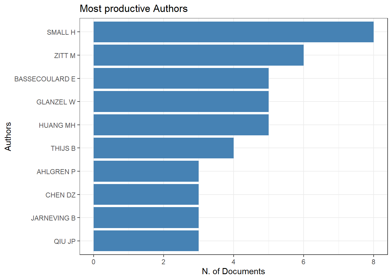
Figure 18.1: Most Productive Authors
18.5.3 Summary Plot-3 (Annual Scientific Production)
p1[[3]]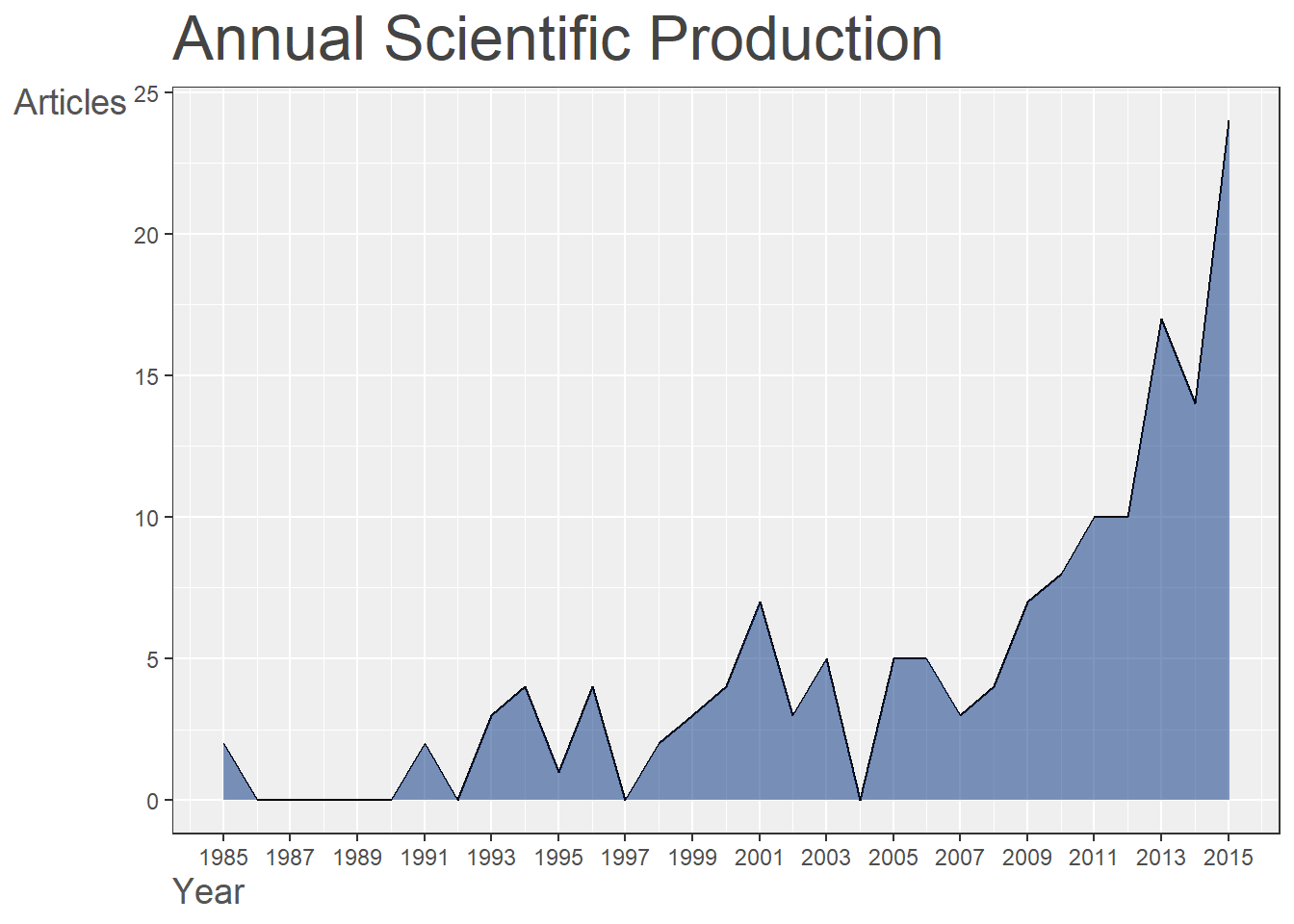
Figure 18.3: Annual Scientific Production
18.5.5 Summary Plot-5 (Author Production Over Time)
A graph for author statistics over time can also be produced.
Figure-17.5 shows a graph of top 10 authors over time. The information from these plots can be easily extracted to summarise them in a table.
topAU = authorProdOverTime(M, k = 10, graph = TRUE)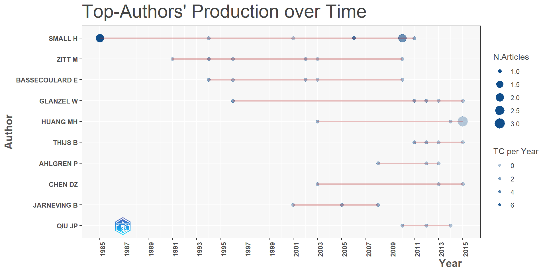
Figure 18.5: Author Production Over Time
18.5.6 Sankey plot
- Bibliometrix provides another useful function to plot a Sankey diagram to visualise multiple attributes at the same time. For example, figure-9 provides a three fields plot for Author, Author Keywords and Cited References.
threeFieldsPlot(M, fields = c("DE", "AU", "AU_CO"))Figure 18.6: Sankey Diagram
18.6 Co-word Analysis
- Analysis of the conceptual structure among the articles analysed.
- Bibliomentrix can conduct a co-word analysis to map the conceptual structure of a framework using the word co-occurrences in a bibliographic database.
- The analysis in Figure-2 is conducted using the Correspondence Analysis and K-Means clustering using Author’s keywords. This analysis includes Natural Language Processing and is conducted without stemming.
library(gridExtra)
CS = conceptualStructure(M, field = "DE", method = "CA", minDegree = 4, clust = "auto",
    stemming = FALSE, labelsize = 8, documents = 10, graph = FALSE)

grid.arrange(CS[[4]], CS[[5]], ncol = 2, nrow = 1)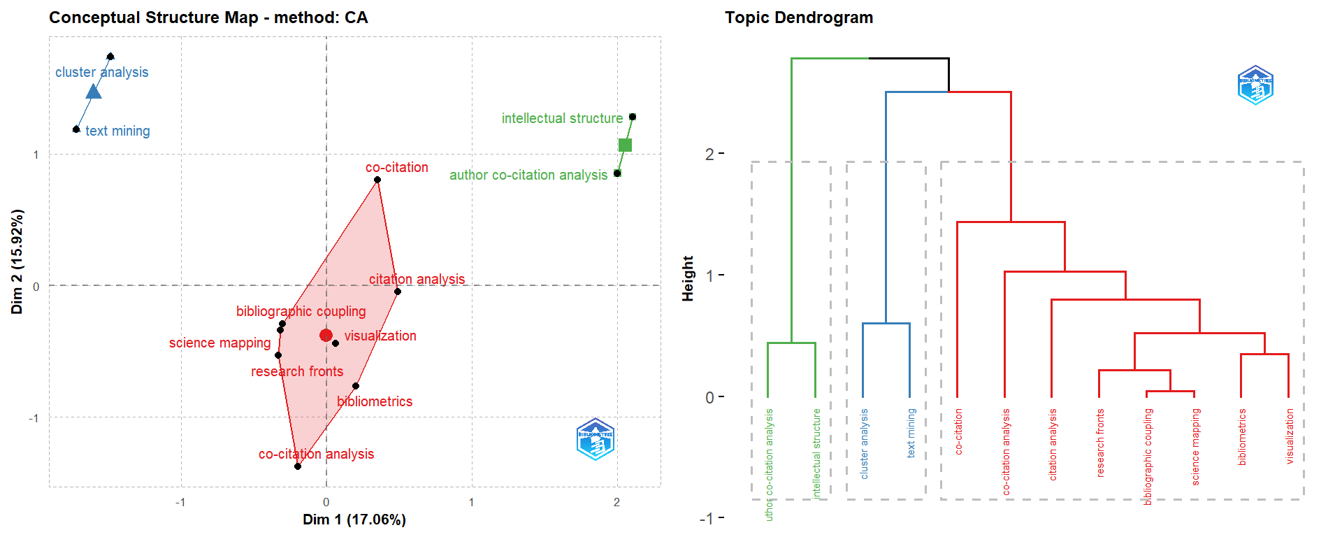
Figure 18.7: Conceptual Structures-1
18.7 Author collaboration network
NetMatrix <- biblioNetwork(M, analysis = "collaboration", network = "authors", sep = ";")
net = networkPlot(NetMatrix, n = 50, Title = "Author collaboration", type = "auto",
    size = 10, size.cex = T, edgesize = 3, labelsize = 0.6)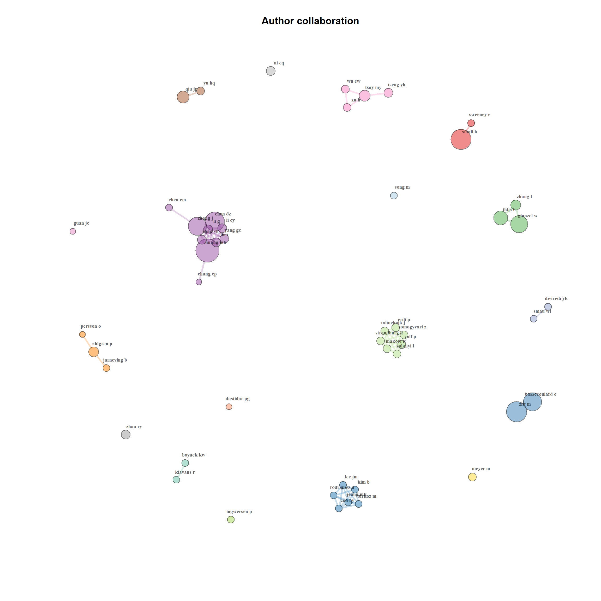
Figure 18.8: Author Collaboration Network
18.8 Keyword co-occurance
Netmatrix2 = biblioNetwork(M, analysis = "co-occurrences", network = "keywords",
    sep = ";")

# Plot the network
net = networkPlot(Netmatrix2, normalize = "association", weighted = T, n = 50, Title = "Keyword Co-occurrences",
    type = "fruchterman", size = T, edgesize = 5, labelsize = 0.7)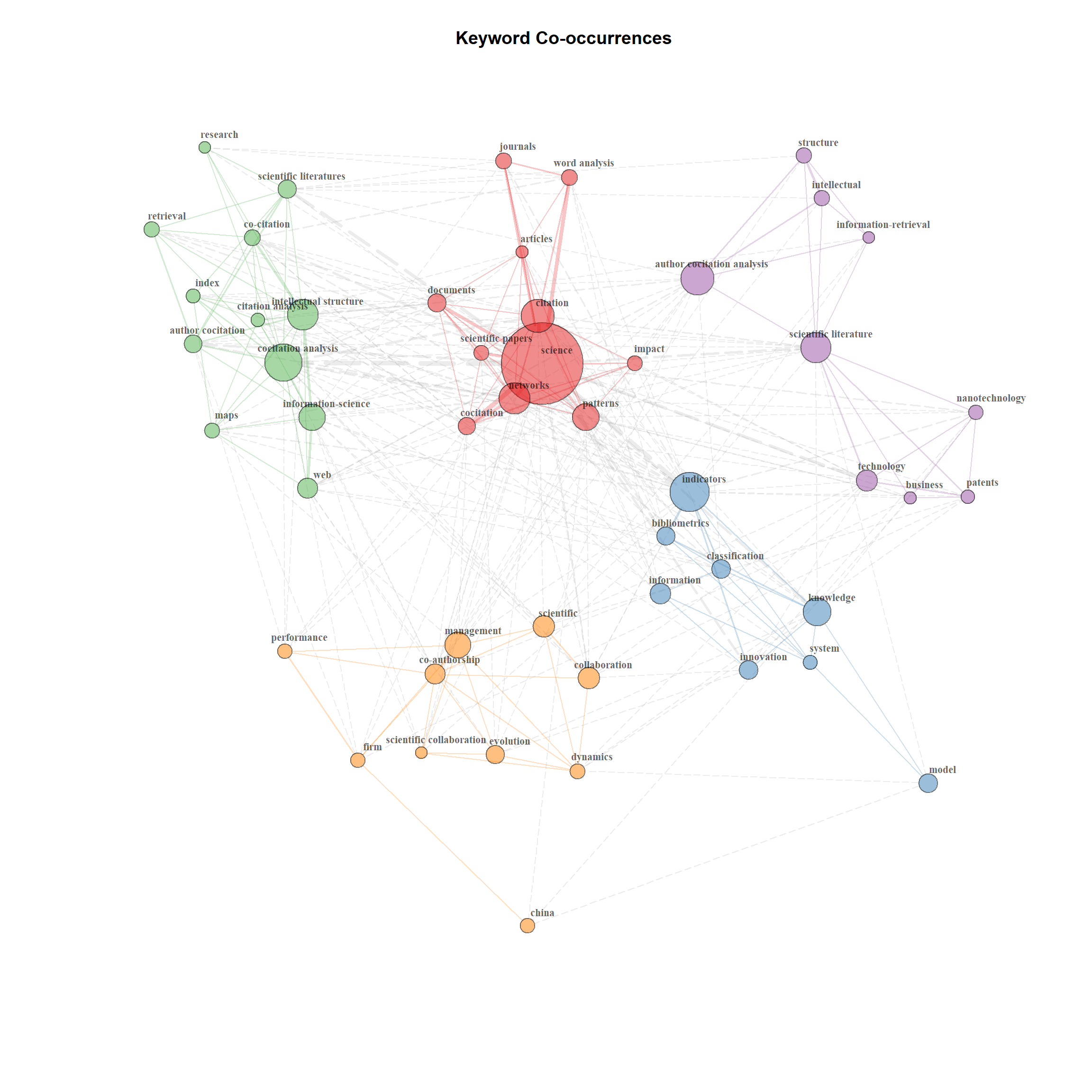
Figure 18.9: Keyword co-occurance
18.9 Thematic Map
Co-word analysis draws clusters of keywords. They are considered as themes, whose density and centrality can be used in classifying themes and mapping in a two-dimensional diagram.
Thematic map is a very intuitive plot and we can analyze themes according to the quadrant in which they are placed: (1) upper-right quadrant: motor-themes; (2) lower-right quadrant: basic themes; (3) lower-left quadrant: emerging or disappearing themes; (4) upper-left quadrant: very specialized/niche themes.
Map = thematicMap(M, field = "ID", n = 1000, minfreq = 5, stemming = FALSE, size = 0.5,
    n.labels = 4, repel = TRUE)
plot(Map$map)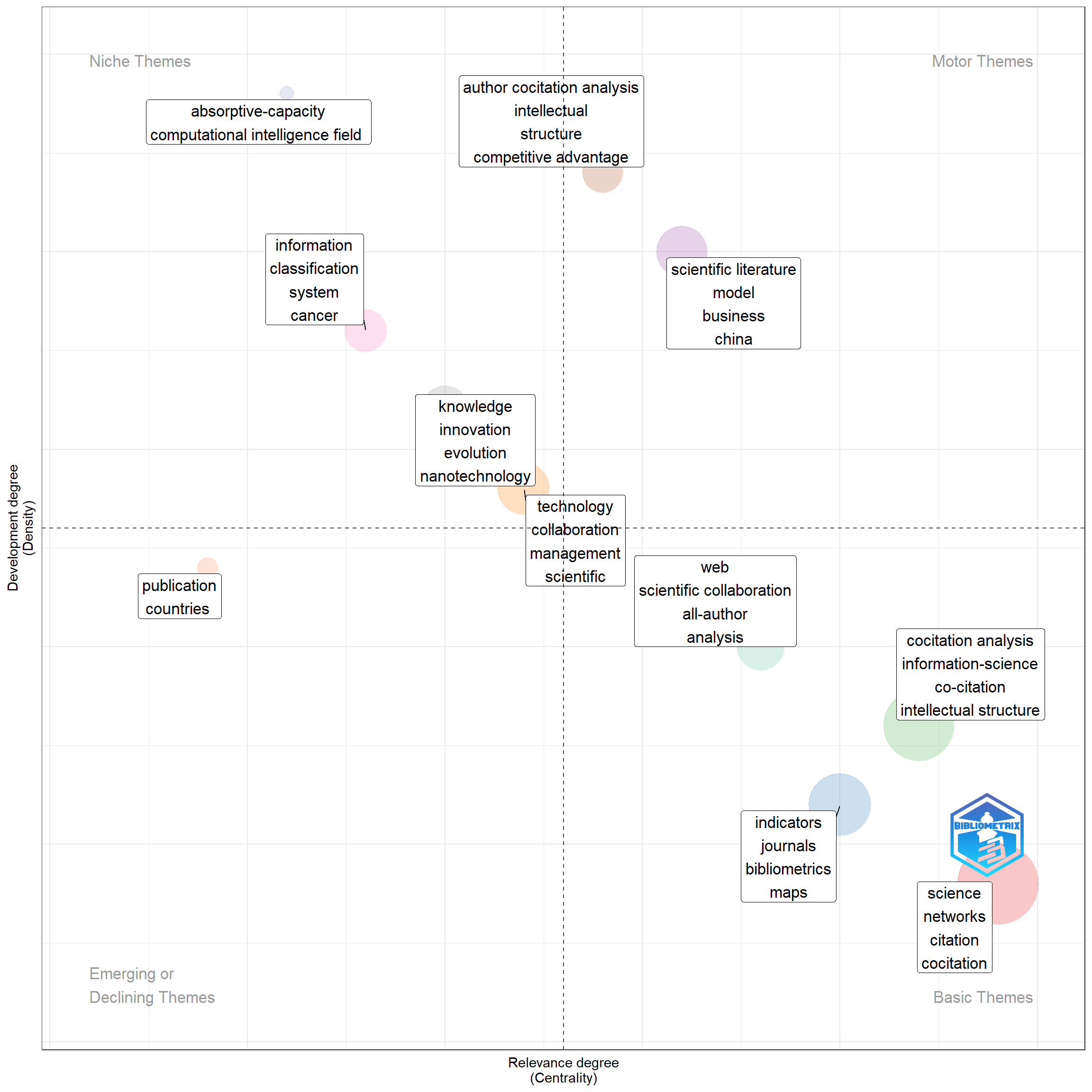
Figure 18.10: Thematic Map
Finally there is a shiny based GUI also available
biblioshiny()