Topic 16 Financial Fraud Analytics

16.1 Introduction to Financial Fraud
Financial institutions deliver several kinds of critical services usually managing high-volume transactions.
Each of these services is afflicted by specific frauds aiming at making illegal profits by unauthorized access to someone’s funds
Earnings manipulation and accounting fraud leads to reduced firm valuation in the long run and a public distrust in the company and its management.
The phenomena of earnings manipulation is not new globally. In 2001, Enron filed for bankruptcy after an accounting fraud resulted in $ 74 billion loss to the shareholders
Firms can manipulate earnings by utilizing their accounting choices known as accrual manipulations.
16.1.1 Types of Financial Fraud
There are various types of financial fraud. The following lists types of financial frauds as listed in Al-Hashedi & Magalingam (2021)
- Credit Card Fraud
- Mortgage Fraud
- Money Laundering
- Financial statement fraud
- Securities and commodities fraud
- Insurance Fraud
- Cryptocurrency Fraud
- Cyber Financial Fraud
16.1.2 ML and AI for Fraud Detection
There are various statistics and ML based classification techniques which are used for detecting fraud. Some of these techniques are
- Support Vector Machines
- Naive Bayes
- Neural Network and Deep Learning
- Random Forests
- Logistic Regression
- KNN
- Decision Trees
- Genetic Algorithms
- Clustering
Ali et al. (2022), Bin Sulaiman, Schetinin, & Sant (2022), Ashtiani & Raahemi (2021), Al-Hashedi & Magalingam (2021), Sadgali, Sael, & Benabbou (2019) provide a review of ML and AI techniques used for financial fraud detection. Bin Sulaiman et al. (2022) provides a review of ML approaches used for Credit Card Fraud Detection.
16.1.3 ML and AI based Fraud Detection System for Credit Card Fraud
Fig-16.1 providesan example of a credit card fraud detection system (source: Le Borgne, Siblini, Lebichot, & Bontempi (2022) Link)
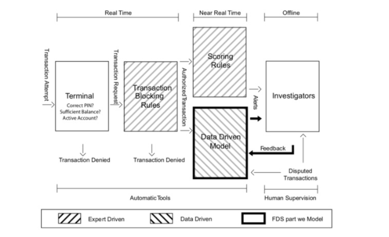
Figure 5.1: Fraud Detection System (Le Borgne et al. (2022))
Next we will discuss a brief example on using ML for Fraud Detection using Labelled data
16.2 Detecting Fraud in Transaction Data
16.2.1 Data
The data is a sample from the simulated transaction dataset availabe on Kaggle.
The kaggle datasets link provides a description of the dataset.
The kaggle dataset is highly unbalanced and requires subsampling techniques like SMOTE.
Chapter-11 of the caret package manual provides a good introduction to subsampling for class imbalances.
The data sample here consists of 10000 observations of 80:20, fraud and no fraud classifications.
Overview of the data
data1 = readRDS("data/fraud_sim.rds")
head(data1)
step type amount nameOrig oldbalanceOrg newbalanceOrig
3193213 247 CASH_OUT 802421.4 C369107118 802421.4 0
6001559 427 TRANSFER 225324.0 C1109518048 225324.0 0
6009616 441 TRANSFER 107363.5 C564631760 107363.5 0
6020272 461 CASH_OUT 1028284.8 C2004363483 1028284.8 0
6034233 476 CASH_OUT 1146381.4 C169415375 1146381.4 0
1030588 74 TRANSFER 4582074.5 C1151172465 4582074.5 0
nameDest oldbalanceDest newbalanceDest isFraud isFlaggedFraud
3193213 C463164064 11846261.7 12648683 1 0
6001559 C1691016675 0.0 0 1 0
6009616 C43570912 0.0 0 1 0
6020272 C165602524 0.0 1028285 1 0
6034233 C1774696541 484779.2 1631161 1 0
1030588 C2088124795 0.0 0 1 0- Data description
- The data consists of 11 attributes
- step: Unit of time, 1 step is 1 hour
- Type: CASH-IN, CASH-OUT, DEBIT, PAYMENT and TRANSFER
- amount: amount of the transaction in local currency
- nameOrg: customer starting the transaction
- oldbalanceorg: initial balance before the transaction
- newlabalanceorig: balance after the transaction
- nameDest: recepient ID of the transaction
- oldBalanceDest: initial recepient balance before the transaction
- newBalanceDest: recepients balance after the transaction
- isFraud: is fradualant (1), not fradualant (0)
- isFlaggedFraud: flags illegal attemps to transfer more that 200,000 units at a time
16.2.2 Summary of the data
library(dplyr)
library(psych)
library(pastecs)
library(tidyr)
library(pander)
pander(stat.desc(data1))| step | type | amount | nameOrig | oldbalanceOrg | |
|---|---|---|---|---|---|
| nbr.val | 10000 | NA | 10000 | NA | 10000 |
| nbr.null | 0 | NA | 3 | NA | 2683 |
| nbr.na | 0 | NA | 0 | NA | 0 |
| min | 1 | NA | 0 | NA | 0 |
| max | 743 | NA | 22925830 | NA | 59585040 |
| range | 742 | NA | 22925830 | NA | 59585040 |
| sum | 2671835 | NA | 4.433e+09 | NA | 9.918e+09 |
| median | 255.5 | NA | 108649 | NA | 31011 |
| mean | 267.2 | NA | 443257 | NA | 991799 |
| SE.mean | 1.67 | NA | 13125 | NA | 30621 |
| CI.mean.0.95 | 3.273 | NA | 25728 | NA | 60022 |
| var | 27878 | NA | 1.723e+12 | NA | 9.376e+12 |
| std.dev | 167 | NA | 1312501 | NA | 3062058 |
| coef.var | 0.6249 | NA | 2.961 | NA | 3.087 |
| newbalanceOrig | nameDest | oldbalanceDest | newbalanceDest | |
|---|---|---|---|---|
| nbr.val | 10000 | NA | 10000 | 10000 |
| nbr.null | 6619 | NA | 4709 | 4038 |
| nbr.na | 0 | NA | 0 | 0 |
| min | 0 | NA | 0 | 0 |
| max | 49585040 | NA | 93819985 | 94779646 |
| range | 49585040 | NA | 93819985 | 94779646 |
| sum | 7.137e+09 | NA | 9.446e+09 | 1.202e+10 |
| median | 0 | NA | 42762 | 195569 |
| mean | 713720 | NA | 944604 | 1202204 |
| SE.mean | 27920 | NA | 28396 | 32128 |
| CI.mean.0.95 | 54729 | NA | 55661 | 62978 |
| var | 7.795e+12 | NA | 8.063e+12 | 1.032e+13 |
| std.dev | 2791998 | NA | 2839565 | 3212822 |
| coef.var | 3.912 | NA | 3.006 | 2.672 |
| isFraud | isFlaggedFraud | |
|---|---|---|
| nbr.val | 10000 | 10000 |
| nbr.null | 8000 | 9996 |
| nbr.na | 0 | 0 |
| min | 0 | 0 |
| max | 1 | 1 |
| range | 1 | 1 |
| sum | 2000 | 4 |
| median | 0 | 0 |
| mean | 0.2 | 4e-04 |
| SE.mean | 0.004 | 2e-04 |
| CI.mean.0.95 | 0.007841 | 0.000392 |
| var | 0.16 | 0.0003999 |
| std.dev | 0.4 | 0.02 |
| coef.var | 2 | 49.99 |
# summarise(data1) %>% select(name,type,na, mean, median, min, max, nlevs)
# summary(data1)- Number of frauds/nofrauds
prop.table(table(data1$isFraud))
  0   1
0.8 0.2
16.2.3 Visualisation
library(ggplot2)
theme_set(theme_minimal())  #globally sets the theme
data1 %>%
    ggplot(aes(isFraud, fill = factor(isFraud))) + geom_bar(stat = "count") + labs(x = "Fraud vs Not Fraud",
    y = "Frequency", fill = "FraudVNon-Fraud")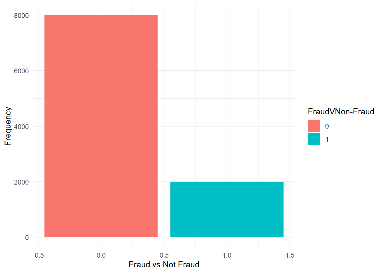
Figure 16.1: FraudVNon-Fraud
- Transactions based on Fraud
data1 %>%
    ggplot(aes(x = type, fill = factor(isFraud))) + geom_bar()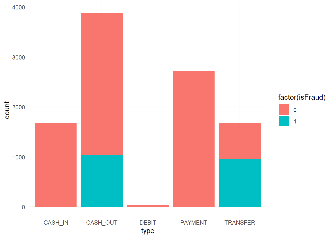
Figure 16.2: Transaction by Fraud
The figure shows that most frauds in the data sample are committed in CASH_OUT of in TRANSFER transaction type
- Distribution of Transactions
library(dplyr)
library(scales)
data1 %>%
    filter(isFraud == 1) %>%
    ggplot(aes(amount)) + geom_histogram() + scale_x_continuous(labels = comma)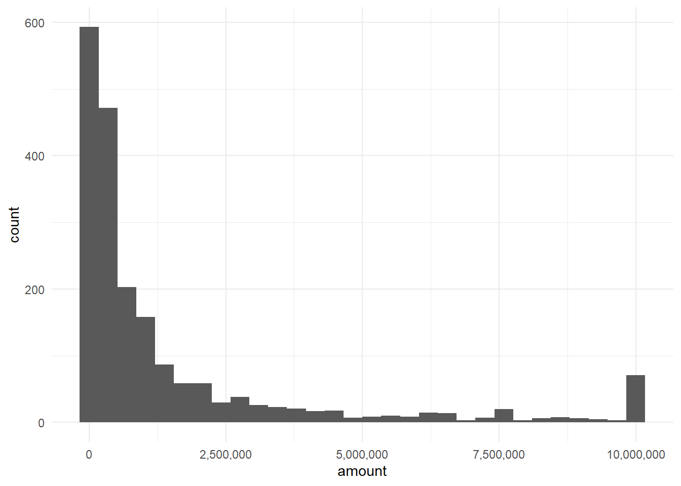
Figure 16.3: Fradualent Amount
- What about balance in accounts?
p1 = data1 %>%
    ggplot(aes(x = factor(isFraud), y = log(oldbalanceOrg), fill = factor(isFraud))) +
    geom_boxplot() + labs(title = "old balance in sender account")
p2 = data1 %>%
    ggplot(aes(x = factor(isFraud), y = log(oldbalanceDest), fill = factor(isFraud))) +
    geom_boxplot() + labs(title = "old balance in receiver account")
library(gridExtra)
grid.arrange(p1, p2, nrow = 1)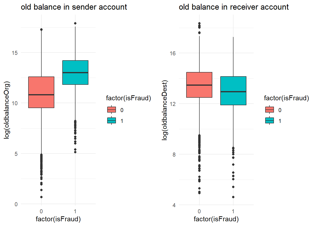
Figure 16.4: Balance (sender/receiver)
Task: Create other visualisations to visually analyse the data
16.3 ML Model
- There are various ML models possible but we will use KNN, Random Forests and Neural Networks
16.3.1 Setup
Select the most useful columns
library(fastDummies)  #for creating dummy columns
data2 = data1 %>%
    select(-c("step", "nameOrig", "nameDest", "isFlaggedFraud")) %>%
    filter(type %in% c("CASH_OUT", "TRANSFER"))
data3 = dummy_cols(data2)  #takes the column with factors and creates dummies based on that
data3$isFraud = as.factor(data3$isFraud)
data3 = data3[, -1]
16.3.2 Sampling and Resampling
- As this is a sample which does not depend on the time series structure, we can use random sampling stratified by the default
library(rsample)
set.seed(123)
idx = initial_split(data3, prop = 0.7, strata = "isFraud")
d_train1 = training(idx)
d_test1 = testing(idx)- Resampling
library(caret)

cntrl1 = trainControl(method = "repeatedcv", number = 10, repeats = 2, allowParallel = TRUE)
prep1 = c("center", "scale", "zv")
16.3.3 KNN
set.seed(123)
mod1_fraud_knn = train(isFraud ~ ., data = d_train1, method = "knn", tuneLength = 10,
preProcess = prep1, trControl = cntrl1)- Model
mod1_fraud_knnk-Nearest Neighbors
3889 samples
7 predictor
2 classes: '0', '1'
Pre-processing: centered (7), scaled (7)
Resampling: Cross-Validated (10 fold, repeated 2 times)
Summary of sample sizes: 3500, 3500, 3500, 3500, 3500, 3500, ...
Resampling results across tuning parameters:
k Accuracy Kappa
5 0.9497300 0.8905007
7 0.9483165 0.8873509
9 0.9466455 0.8834357
11 0.9458736 0.8816692
13 0.9429167 0.8750019
15 0.9411165 0.8707704
17 0.9381596 0.8640186
19 0.9368746 0.8611598
21 0.9343039 0.8554145
23 0.9328887 0.8522490
Accuracy was used to select the optimal model using the largest value.
The final value used for the model was k = 5.- Predictive Accuracy
set.seed(123)
pred1 = predict(mod1_fraud_knn, newdata = d_test1)
confusionMatrix(pred1, d_test1$isFraud)
Confusion Matrix and Statistics
Reference
Prediction 0 1
0 1026 50
1 41 550
Accuracy : 0.9454
95% CI : (0.9334, 0.9558)
No Information Rate : 0.6401
P-Value [Acc > NIR] : <2e-16
Kappa : 0.8811
Mcnemar's Test P-Value : 0.4017
Sensitivity : 0.9616
Specificity : 0.9167
Pos Pred Value : 0.9535
Neg Pred Value : 0.9306
Prevalence : 0.6401
Detection Rate : 0.6155
Detection Prevalence : 0.6455
Balanced Accuracy : 0.9391
'Positive' Class : 0
16.3.4 Random Forests
mtry = sqrt(ncol(d_test1))
tunegrid = expand.grid(.mtry = mtry)
library(doParallel)
cl = makePSOCKcluster(detectCores()/2)
registerDoParallel(cl)
set.seed(123)


rf_fraud = train(isFraud ~ ., data = d_train1, method = "rf", tuneGrid = tunegrid,
    trControl = cntrl1, preProcess = prep1)
stopCluster(cl)
registerDoSEQ()- Model
rf_fraudRandom Forest
3889 samples
7 predictor
2 classes: '0', '1'
Pre-processing: centered (7), scaled (7)
Resampling: Cross-Validated (10 fold, repeated 2 times)
Summary of sample sizes: 3500, 3500, 3500, 3500, 3500, 3500, ...
Resampling results:
Accuracy Kappa
0.9755708 0.9469659
Tuning parameter 'mtry' was held constant at a value of 2.828427- Predictive Accuracy
set.seed(123)
pred2 = predict(rf_fraud, newdata = d_test1)
confusionMatrix(pred2, d_test1$isFraud)
Confusion Matrix and Statistics
Reference
Prediction 0 1
0 1049 15
1 18 585
Accuracy : 0.9802
95% CI : (0.9723, 0.9863)
No Information Rate : 0.6401
P-Value [Acc > NIR] : <2e-16
Kappa : 0.9571
Mcnemar's Test P-Value : 0.7277
Sensitivity : 0.9831
Specificity : 0.9750
Pos Pred Value : 0.9859
Neg Pred Value : 0.9701
Prevalence : 0.6401
Detection Rate : 0.6293
Detection Prevalence : 0.6383
Balanced Accuracy : 0.9791
'Positive' Class : 0
16.3.5 NNET
library(doParallel)
cl = makePSOCKcluster(detectCores()/2)
registerDoParallel(cl)
set.seed(123)


nnet_fraud = train(isFraud ~ ., data = d_train1, method = "nnet", trControl = cntrl1,
    preProcess = prep1)
# weights: 28
initial value 2899.085170
iter 10 value 1454.628563
iter 20 value 537.562073
iter 30 value 332.100069
iter 40 value 189.749918
iter 50 value 152.552874
iter 60 value 112.587854
iter 70 value 106.284558
iter 80 value 98.840062
iter 90 value 95.032644
iter 100 value 93.058743
final value 93.058743
stopped after 100 iterationsstopCluster(cl)
registerDoSEQ()- Model
nnet_fraudNeural Network
3889 samples
7 predictor
2 classes: '0', '1'
Pre-processing: centered (7), scaled (7)
Resampling: Cross-Validated (10 fold, repeated 2 times)
Summary of sample sizes: 3500, 3500, 3500, 3500, 3500, 3500, ...
Resampling results across tuning parameters:
size decay Accuracy Kappa
1 0e+00 0.9805866 0.9575230
1 1e-04 0.9820012 0.9610373
1 1e-01 0.9553895 0.9021244
3 0e+00 0.9845725 0.9665263
3 1e-04 0.9822559 0.9615537
3 1e-01 0.9628459 0.9186841
5 0e+00 0.9832875 0.9636761
5 1e-04 0.9823854 0.9618194
5 1e-01 0.9633603 0.9197440
Accuracy was used to select the optimal model using the largest value.
The final values used for the model were size = 3 and decay = 0.- Predictive Accuracy
set.seed(123)
pred3 = predict(nnet_fraud, newdata = d_test1)
confusionMatrix(pred3, d_test1$isFraud)
Confusion Matrix and Statistics
Reference
Prediction 0 1
0 1060 9
1 7 591
Accuracy : 0.9904
95% CI : (0.9845, 0.9945)
No Information Rate : 0.6401
P-Value [Acc > NIR] : <2e-16
Kappa : 0.9792
Mcnemar's Test P-Value : 0.8026
Sensitivity : 0.9934
Specificity : 0.9850
Pos Pred Value : 0.9916
Neg Pred Value : 0.9883
Prevalence : 0.6401
Detection Rate : 0.6359
Detection Prevalence : 0.6413
Balanced Accuracy : 0.9892
'Positive' Class : 0