Topic 17 Text Mining using R

“We Facebook users have been building a treasure lode of big data that government and corporate researchers have been mining to predict and influence what we buy and for whom we vote. We have been handing over to them vast quantities of information about ourselves and our friends, loved ones and acquaintances”-Douglas Rushkoff
17.1 Introduction to Text Mining
Text mining, also referred to as text data mining, roughly equivalent to text analytics, refers to the process of deriving high-quality information from text. High-quality information is typically derived through the devising of patterns and trends through means such as statistical pattern learning.
Welbers et al. (2017) provides a mild introduction to Text Analytics using R
Text mining has gained momentum and is used in analytics worldwide
Sentiment Analysis
Predicting Stock Market and other Financial Applications
Customer influence
News Analytics
Social Network Analysis
Customer Service and Help Desk
17.1.1 Text Data
Text data is ubiquitous in social media analytics.
Traditional media, social media, survey data, and numerous other sources.
- Twitter, Facebook, Surveys, Reported Data (Incident Reports)
Massive quantity of text in the modern information age.
The mounting availability of and interest in text data has been the development of a variety of statistical approaches for analysing this data.
17.1.2 Generic Text Mining System
- Following figure demonstrates a general text mining system (Source: Feldman & Sanger (2007))
knitr::include_graphics("fig-2.png")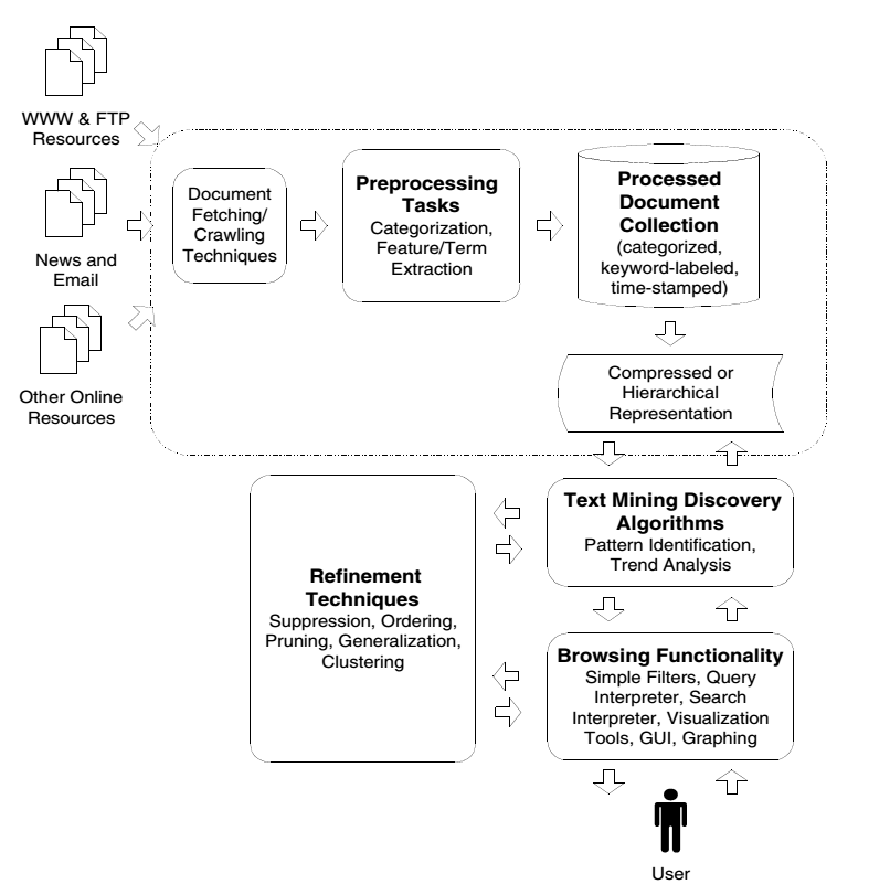
Figure 17.1: Generic Text Mining System
17.2 Mining Twitter Text Data using R
Twitter is one of the most popular social media platform for information sharing. Some examples from rforresearch tweets Follow (rforresearch?) Tweets by rforresearch17.2.1 Obtaining Twitter Data
Twitter provides an API access for their data feed.
User is required to create an app and obtain access codes for the API.
See here https://cran.r-project.org/web/packages/rtweet/vignettes/auth.html for a detailed introduction on obtaining API credentials.
Data access is limited in various ways (days, size of data etc.).
See here https://developer.twitter.com/en/docs.html for full documentation.
R provides packages like twitteR and rtweet provide programming interface using R to access the data.
Twitter doesnt allow data sharing but the API setup is straight forward. Twitter does allow sharing of the tweet IDs (available in the data folder)
17.3 Download Data
- We will download tweets with ‘#auspol’; a popular hashtag used in Australia to talk about current affairs and socio-political issues
- Example here uses rtweet package to download data
- After setting up the API
- Create the token
search_tweetscan be used without creating the token, it will create a token using the default app for your Twitter account
library(rtweet)

token <- create_token(app = "your_app_name", consumer_key = "your_consumer_key",
    consumer_secret = "your_consumer_secret", access_token = "your_access_token",
access_secret = "your_access_secret")- Use the
search_tweetsfunction to download the data, convert to data frame and save
rt = search_tweets(q = "#auspol", n = 15000, type = "recent", include_rts = FALSE,
since = "2020-09-14")
rt2 = as.data.frame(rt)
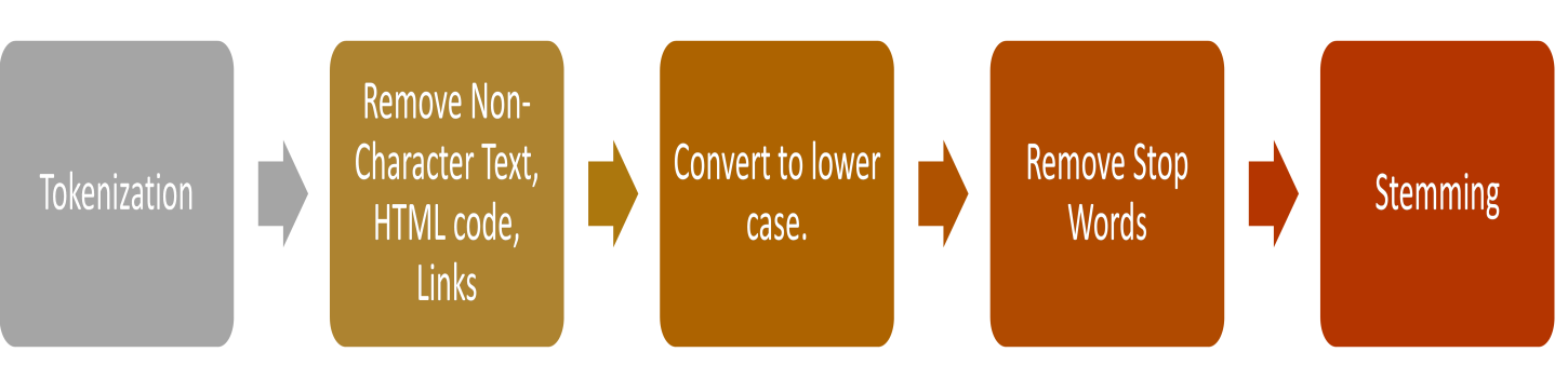
saveRDS(rt2, file = "tweets_auspol.rds")17.4 Data Pre-processing
We will conduct data pre-processing in this stage
Some steps (depend on the types of problems analysed)
- Create a corpus
- Change encoding
- Convert to lower case
- Remove hashtags
- Remove URLs
- Remove @ mentions
- Remove punctuations
- Remove stop words
- Stemming can also be conducting (avoided in this example)
library(tm)
rt = readRDS("tweets_auspol.rds")
# encoding
rt$text <- sapply(rt$text, function(row) iconv(row, "latin1", "ASCII", sub = ""))

# build a corpus, and specify the source to be character vectors

myCorpus = Corpus(VectorSource(rt$text))


# convert to lower case
myCorpus = tm_map(myCorpus, content_transformer(tolower))
# remove punctuation
myCorpus <- tm_map(myCorpus, removePunctuation)
# remove numbers
myCorpus <- tm_map(myCorpus, removeNumbers)


# remove URLs
removeURL = function(x) gsub("http[^[:space:]]*", "", x)
removeURLs = function(x) gsub("https[^[:space:]]*", "", x)

# remove hashtags

removehash = function(x) gsub("#\\S+", "", x)

# remove @
removeats <- function(x) gsub("@\\w+", "", x)  #only removes the '@'

# remove numbers and punctuations
removeNumPunct = function(x) gsub("[^[:alpha:][:space:]]*", "", x)

# leading and trailing white spaces

wspace1 = function(x) gsub("^[[:space:]]*", "", x)  ## Remove leading whitespaces
wspace2 = function(x) gsub("[[:space:]]*$", "", x)  ## Remove trailing whitespaces
wspace3 = function(x) gsub(" +", " ", x)  ## Remove extra whitespaces

removeIms <- function(x) gsub("im", "", x)

myCorpus = tm_map(myCorpus, content_transformer(removeURL))  #url
myCorpus = tm_map(myCorpus, content_transformer(removeURLs))  #url

myCorpus <- tm_map(myCorpus, content_transformer(removehash))  #hashtag
myCorpus <- tm_map(myCorpus, content_transformer(removeats))  #mentions

myCorpus = tm_map(myCorpus, content_transformer(removeNumPunct))  #number and punctuation (just in case some are left over)

myCorpus = tm_map(myCorpus, content_transformer(removeIms))  #Ims

myCorpus = tm_map(myCorpus, content_transformer(wspace1))
myCorpus = tm_map(myCorpus, content_transformer(wspace2))
myCorpus = tm_map(myCorpus, content_transformer(wspace3))  #other white spaces

# remove extra whitespace
myCorpus = tm_map(myCorpus, stripWhitespace)

# remove extra stopwords
myStopwords = c(stopwords("English"), stopwords("SMART"), "rt", "ht", "via", "amp",
    "the", "australia", "australians", "australian", "auspol")

myCorpus = tm_map(myCorpus, removeWords, myStopwords)

# generally a good idea to save the processed corpus now
save(myCorpus, file = "auspol_sep.RData")

data_tw2 = data.frame(text = get("content", myCorpus), row.names = NULL)
data_tw2 = cbind(data_tw2, ID = rt$status_id)
data_tw2 = cbind(Date = as.Date(rt$created_at), data_tw2)
# look at the data frame, still some white spaces left so let's get rid of them
data_tw2$text = gsub("\r?\n|\r", "", data_tw2$text)
data_tw2$text = gsub(" +", " ", data_tw2$text)
head(data_tw2)
# save data
saveRDS(data_tw2, file = "processed_data.rds")
17.5 Some Visualisation
- Bar Chart of top words
library(tm)
load("auspol_sep.RData")
# Build TDM
tdm = TermDocumentMatrix(myCorpus, control = list(wordLengths = c(3, Inf)))
m = as.matrix(tdm)
word.freq = sort(rowSums(m), decreasing = T)
# plot term freq
term.freq1 = rowSums(as.matrix(tdm))
term.freq = subset(term.freq1, term.freq1 >= 50)
df = data.frame(term = names(term.freq), freq = term.freq)
df = transform(df, term = reorder(term, freq))
library(ggplot2)
library(ggthemes)

m2 = ggplot(head(df, n = 20), aes(x = reorder(term, -freq), y = freq)) + geom_bar(stat = "identity",
    aes(fill = term)) + theme(legend.position = "none") + ggtitle("Top 20 words in tweets #auspol \n (14 Sep to 20 Sep 2020)") +
    theme(axis.text = element_text(size = 12, angle = 90, face = "bold"), axis.title.x = element_blank(),
        title = element_text(size = 15))
m2 = m2 + xlab("Words") + ylab("Frequency") + theme_wsj() + theme(legend.position = "none",
    text = element_text(face = "bold", size = 10))
m2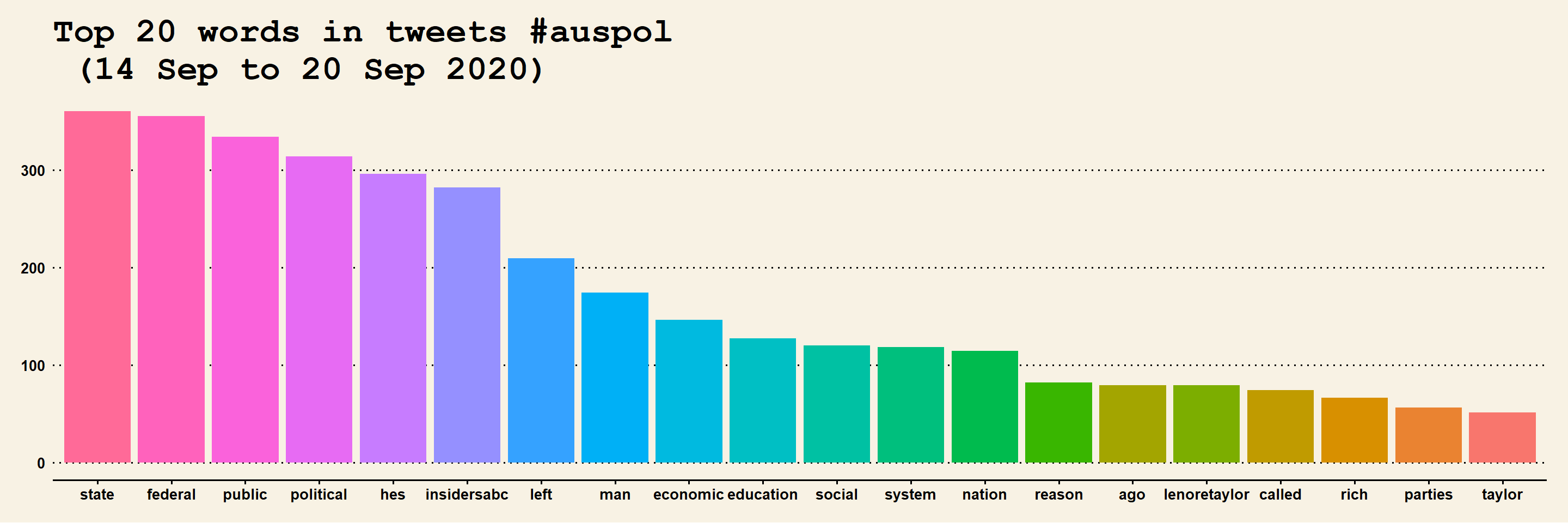
Figure 17.3: Top 20 Words
- Word Cloud 1
library(wordcloud)
library(RColorBrewer)
pal = brewer.pal(7, "Dark2")
wordcloud(words = names(word.freq), freq = word.freq, min.freq = 5, max.words = 1000,
    random.order = F, colors = pal)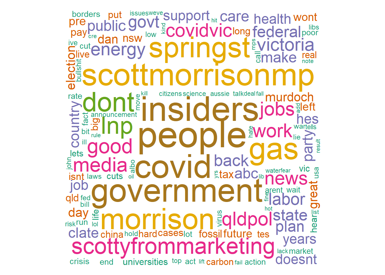
Figure 17.4: Wordcloud-1
- Word Cloud 2
library(wordcloud2)
# some data re-arrangement
term.freq2 = data.frame(word = names(term.freq1), freq = term.freq1)
term.freq2 = term.freq2[term.freq2$freq > 5, ]
# figure-3.4
wordcloud2(term.freq2)
Figure 17.5: Wordcloud-2
The word cloud reflects the discussion around the Federal Government’s new Energy Policy announced during the data time period
17.6 Sentiment Analysis
Classification of Sentiment Analysis Methods
17.6 shows various classification of sentiment analysis methods (Collomb, Costea, Joyeux, Hasan, & Brunie (2014))
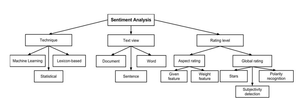
Figure 17.6: Classification of Sentiment Analysis Methods
17.6.1 Method
Lexicon (or Dictionary) based method used in the following illustration.
Sentence level classification
Eight emotions to classify: “anger, fear, anticipation, trust, surprise, sadness, joy, and disgust”
Lexicon Used: NRC Emotion Lexicon.
See http://saifmohammad.com/WebPages/NRC-Emotion-Lexicon.htm
See Mohammad & Turney (2010) for more details on the lexicon.
# required libraries sentiment analysis
library(syuzhet)
library(lubridate)
library(ggplot2)
library(scales)
library(reshape2)
library(dplyr)
library(qdap)
# convert data to dataframe for analysis
data_sent = readRDS("processed_data.rds")
data_sent = data_sent[!apply(data_sent, 1, function(x) any(x == "")), ]  #remove rows with empty values
data_sent = data_sent[wc(data_sent$text) > 4, ]  #more than 4 words per tweet
tw2 = data_sent$text- Conduct Sentiment Analysis and Visualise
mySentiment = get_nrc_sentiment(tw2)  #this can take some time
tweets_sentiment = cbind(data_sent, mySentiment)
# save the results
saveRDS(tweets_sentiment, file = "tw_sentiment.rds")- Plot
sentimentTotals = data.frame(colSums(tweets_sentiment[, c(4:13)]))
names(sentimentTotals) = "count"
sentimentTotals = cbind(sentiment = rownames(sentimentTotals), sentimentTotals)
rownames(sentimentTotals) = NULL
# plot
ggplot(data = sentimentTotals, aes(x = sentiment, y = count)) + geom_bar(aes(fill = sentiment),
    stat = "identity") + theme(legend.position = "none") + xlab("Sentiment") + ylab("Total Count") +
    ggtitle("Sentiment Score for Sample Tweets") + theme_minimal() + theme(axis.text = element_text(size = 15,
    face = "bold"))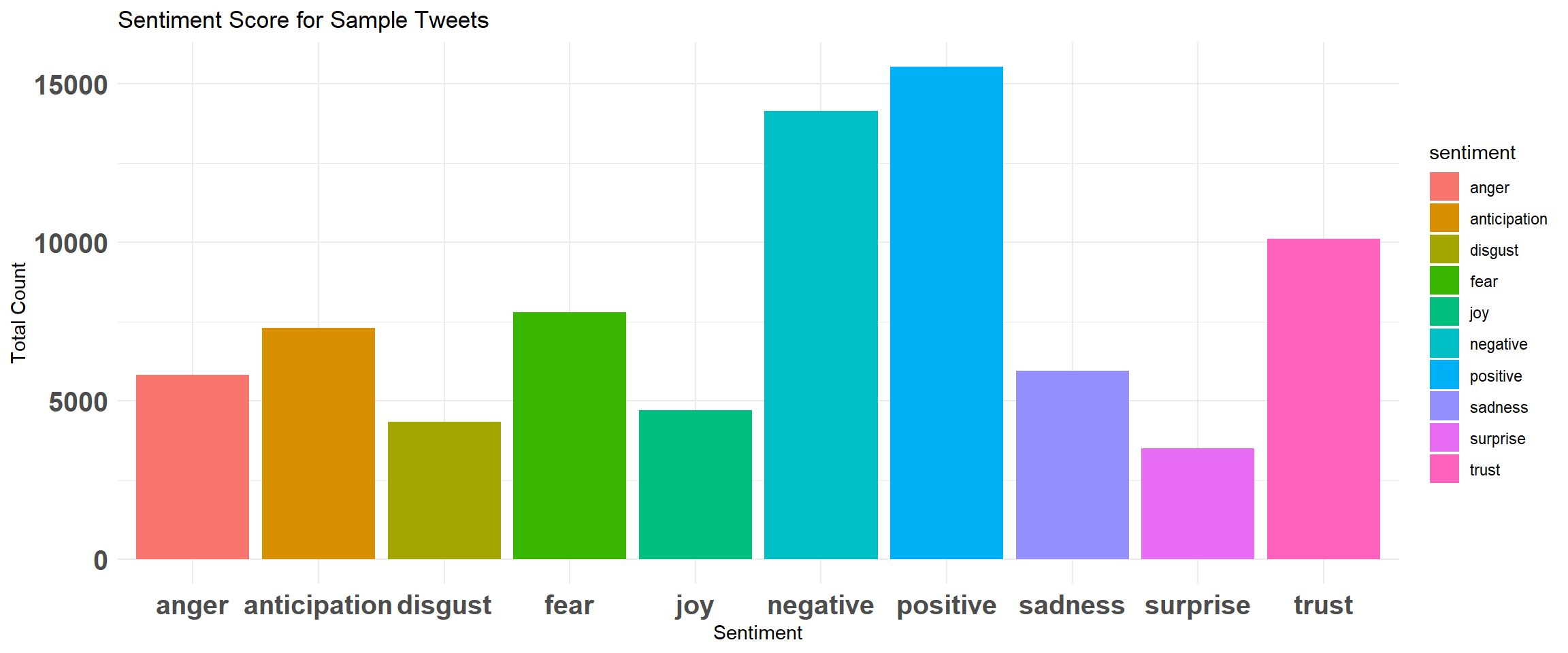
Figure 17.7: Emotions/Sentiment Scores
17.7 Topic Modelling
This section will use bi-term topic modelling method to demonstrate topic modelling exercise.
Biterm Topic Modelling (BTM) (Yan, Guo, Lan, & Cheng (2013)) is useful for short text like the twitter data we have in this example.
- A BTM is a word co-occurance based topic model that learns topics by modelling word-word patterns (biterms)
- BTM models biterm occurences in a corpus
- More details here https://github.com/xiaohuiyan/xiaohuiyan.github.io/blob/master/paper/BTM-WWW13.pdf
- A good example here http://www.bnosac.be/index.php/blog/98-biterm-topic-modelling-for-short-texts
# load packages and rearrange data
library(udpipe)
library(data.table)
library(stopwords)
library(BTM)
library(textplot)
library(ggraph)
# rearrange to get doc id
data_tm = data_sent[, c(3, 2)]
colnames(data_tm)[1] = "doc_id"
# use parts of sentence (Nouns, Adjectives, Verbs for TM) Method is
# computationally intensive and can take several minutes.
anno <- udpipe(data_tm, "english", trace = 1000)
biterms <- as.data.table(anno)
biterms <- biterms[, cooccurrence(x = lemma, relevant = upos %in% c("NOUN", "ADJ",
"VERB") & nchar(lemma) > 2 & !lemma %in% stopwords("en"), skipgram = 3), by = list(doc_id)]
set.seed(999)
traindata <- subset(anno, upos %in% c("NOUN", "ADJ", "VERB") & !lemma %in% stopwords("en") &
nchar(lemma) > 2)
traindata <- traindata[, c("doc_id", "lemma")]
# fit 10 topics (other parameters are mostly default)
model <- BTM(traindata, biterms = biterms, k = 10, iter = 2000, background = FALSE,
trace = 2000)
# extract biterms for plotting
biterms1 = terms(model, type = "biterms")$biterms
# The model, biterms, biterms1 were saved to create the plot in this markdown
# document.- Plot the topics with 20 terms and labelled by the proportion
plot(model, subtitle = "#auspol 14-20 Sep 2020", biterms = biterms1, labels = paste(round(model$theta *
    100, 2), "%", sep = ""), top_n = 20)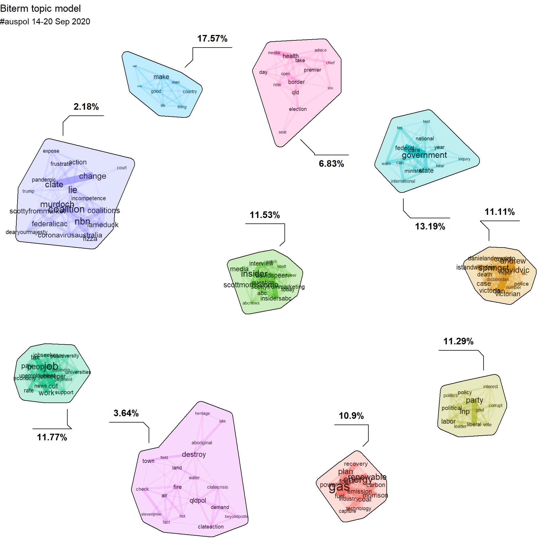
Figure 17.8: BTM Visualisation of #auspol
- Other analysis which can be conducted may include, clustering analysis, co-word clusters, network analysis etc. Other Topic Modelling methods can also be implemented.