Topic 5 Graphics in R (Part-I)
5.1 Basic Plots in R
5.1.1 Scatter Plot
- One of the most popular and most frequently used functions to build a new plot in R is the \(\mathtt{plot}\) function.
- Plot is a high level generic graphic function which depends on the class of the first argument (usually the data object). For example if the first argument is of the class zoo which is a timeseries object the \(\mathtt{plot}\) function will call \(\mathtt{plot.zoo}\) from the R package zoo. This time series plot can be a single timeseries line plot or multiple time series stacked plot.
# Generate two random normal vectors
x = rnorm(100)
y = rnorm(100)
# plot x and y using the plot() function
plot(x, y)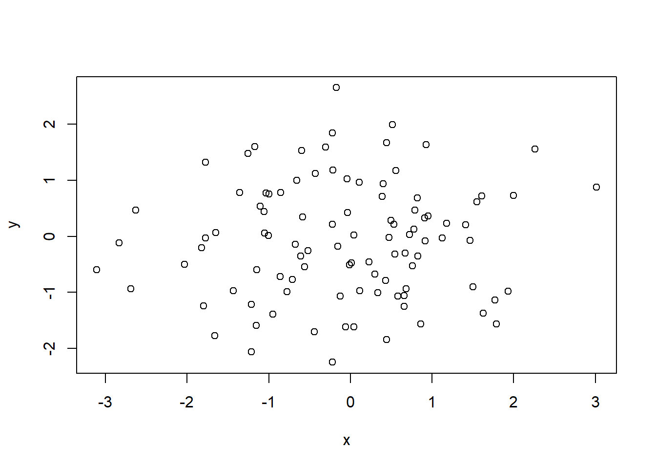
Figure 5.1: Simple Scatter Plot
- There are various other arguments which can be modified to change the overall presentation of the plot and even the type of plot.
args(plot.default)function (x, y = NULL, type = "p", xlim = NULL, ylim = NULL,
log = "", main = NULL, sub = NULL, xlab = NULL, ylab = NULL,
ann = par("ann"), axes = TRUE, frame.plot = axes, panel.first = NULL,
panel.last = NULL, asp = NA, xgap.axis = NA, ygap.axis = NA,
...)
NULL- The following example uses the argument \(\mathtt{main}\) in the \(\mathtt{plot}\) function to include a title on the plot along with axis tiles using the arguments \(\mathtt{xlab}\) and \(\mathtt{ylab}\).
plot(x, y, main = "Figure-2", xlab = "Normal X", ylab = "Normal Y")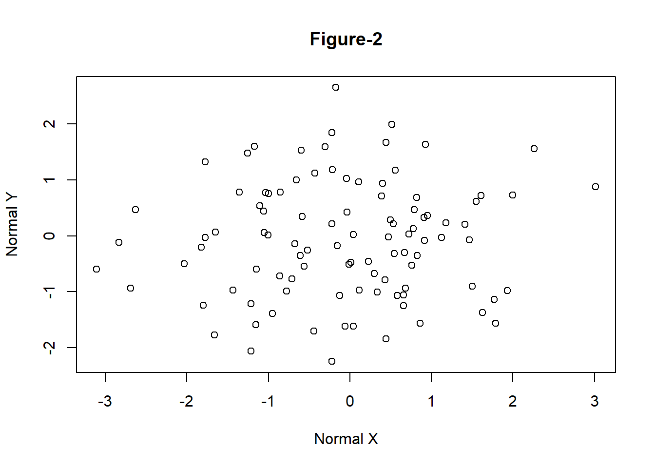
Figure 5.2: Simple Scatter Plot with Title
5.1.2 Line Plot
- The following example demonstrates how to create a line plot using Microsoft prices given in the data file \(\mathtt{data\_fin.RData}\).
# change the working directory to the folder containing data_fin.csv or provide
# the full path with the filename
load("data/data_fin.RData")
# column names
colnames(FinData)
[1] "Date" "DJI" "AXP" "MMM" "ATT" "BA" "CAT" "CISCO" "DD"
[10] "XOM" "GE" "GS" "HD" "IBM" "INTC" "JNJ" "JPM" "MRK"
[19] "MCD" "MSFT" "NKE" # plot a line plot for Dow Jones stock index prices
plot(FinData$MSFT, type = "l", main = "Microsoft Prices", ylab = "Prices")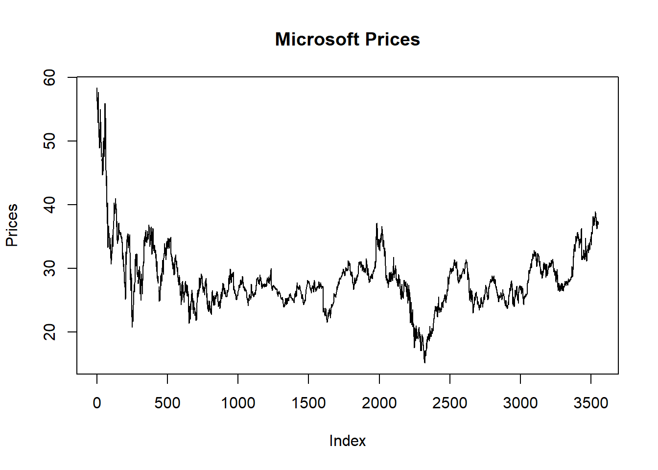
Figure 5.3: Line Chart
- Plotting it as Time Series data
- Various R packages provide functionality to plot specific data types. For example, \(\mathtt{zoo}\) can be used to plot time series data.
library(zoo)
# convert data to class zoo
FinData.ts = zoo(FinData[, 2:5], order.by = FinData$Date)
# plot multiple stacked plot
plot(FinData.ts, col = gray.colors(4))  #figure-4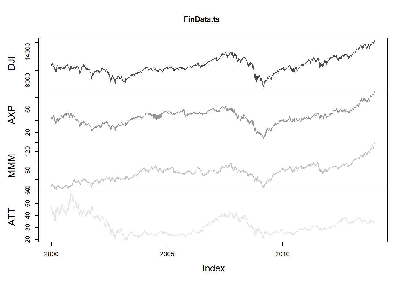
Figure 5.4: Time Series Plot
5.1.3 Bar Plot
- The function \(\mathtt{barplot}\) creates bar graphs in R.
- The main data argument in this function is \(\mathtt{height}\) which can be a vector or a matrix of values describing the bars which make up the plot. If \(\mathtt{height}\)is a matrix the bar graph can be a stacked graph or a juxtaposed graph with \(\mathtt{besides=TRUE}\)
load("data/GDP_Yearly.RData")
par1 = par()
par(ask = F)
barplot(height = GDP$Australia, names.arg = GDP$Year, ylab = "GDP Per Capita")  #figure-5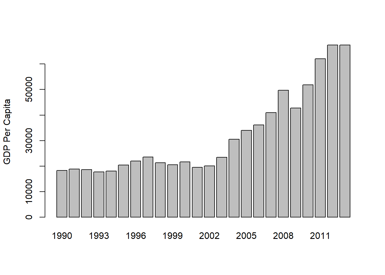
Figure 5.5: Bar Graph with argument height as vector
It is also possible to create a yearly vertical stacked or yearly horizontal grouped bar plot for the GDP data.
The data has to be first converted into a matrix to create stacked or grouped barplots.
In this example the argument \(\mathtt{legend}\) specifies the names (Years) to appear in the legend and the argument \(\mathtt{args.legend}\) specifies the position (x=”top”), alignment (horiz=TRUE) and distance from the margin (inset=-0.1).
# convert data to matrix
data = as.matrix(GDP[, 2:12])
# create row names
rownames(data) = GDP$Year
# plot a stacked bar plot with legend showing the years
barplot(height = data[1:5, ], beside = FALSE, col = rainbow(5), legend = rownames(data[1:5,
    ]), args.legend = list(x = "top", horiz = TRUE, inset = -0.1), cex.names = 0.6)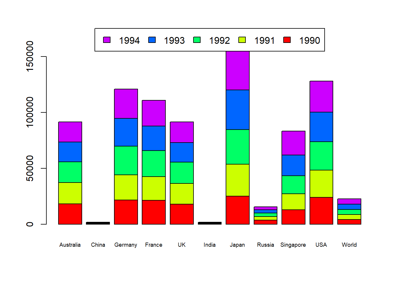
Figure 5.6: Vertical Stacked Barplot
par(par1)5.1.4 Pie Chart
- R provides the function \(\mathtt{pie}\) to create pie graphs. \(\mathtt{labels}\) in 5.7
pie(x = data[1, ], labels = colnames(data))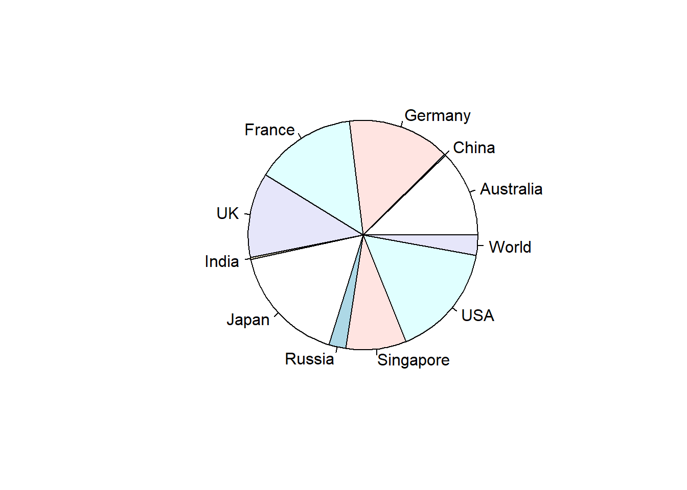
Figure 5.7: Pie Chart
5.1.5 Scatter Plot
- The basic \(\mathtt{plot}\) function plots a scatter plot for bivariate or univariate data. It is also possible to create a scatterplot for multivariate data using the \(\mathtt{pairs}\) function.
pairs(data[, 1:5])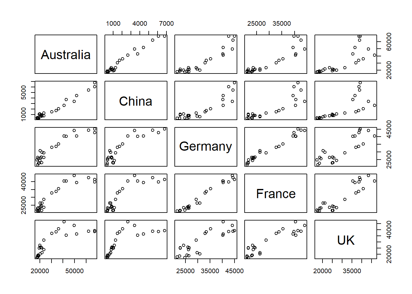
Figure 5.8: Scatterplot
- A subset can also be selected using formula method, for example the following R code will generate a scatterplot with only Australia, UK and USA.
pairs(~Australia + UK + USA, data = data)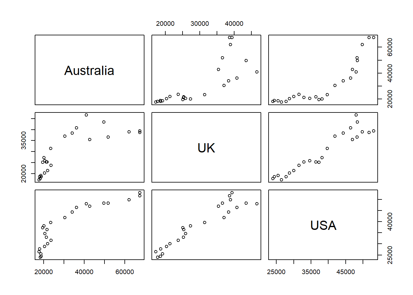
Figure 5.9: Scatterplot (subset)
5.2 R Graphical Parameters
The \(\mathtt{par}\) function facilitates access and modification of a large list of parameters such as color, margin, number of rows and columns on a graphic device etc (see \(\mathtt{help(par)}\) for a list of such parameters).
R provides various margin parameters to tweak inner and outer margins of a graphical device.
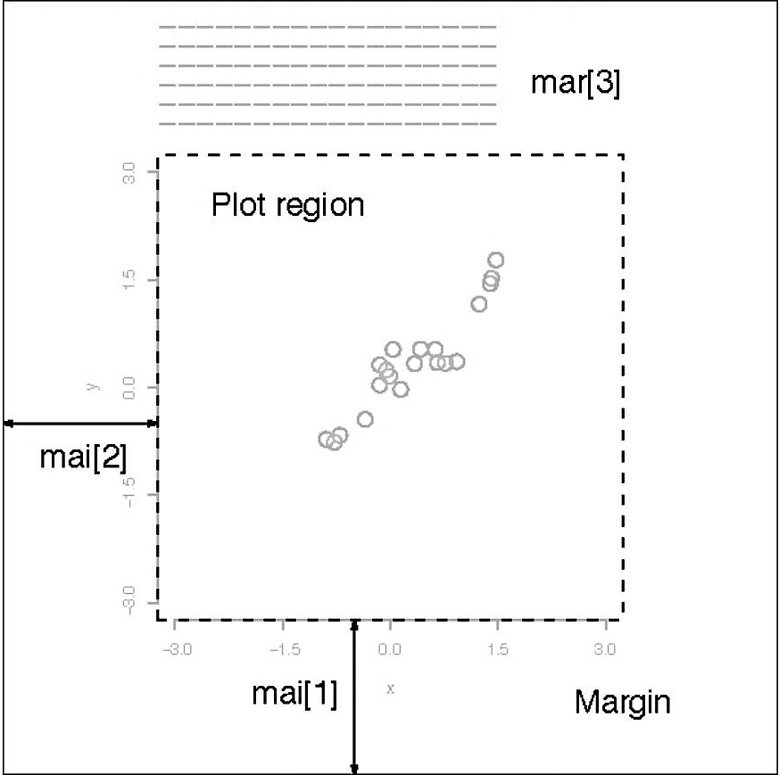
Figure 5.10: Graph Margins
A modification to par always changes the global values of graphic parameters and hence its is a good practice to first store the default parameters in a separate object (variable) which can be later used to restore default graphic parameters.
These margins can be altered using or parameters with the first setting the margins in inches and the second in unit of text lines. Setting one of these will adjust the other accordingly.
The following example (output not shown here) changes the margins to \(\mathtt{c(5,4,7,2)}\) from the default of \(\mathtt{c(5,4,4,2)+0.1}\) to accommodate a title on top of the figure.
# first save the default parameters
par.old = par()
# change the margins
par(mar = c(5, 4, 7, 2))
# plot the bargraph
barplot(height = data[1:5, ], beside = FALSE, col = rainbow(5), legend = rownames(data[1:5,
    ]), args.legend = list(x = "top", horiz = TRUE, inset = -0.1), cex.names = 0.6)
title("Bar Plot \n(with custom margins)")
# set parameters to default
par(par.old)- A multiple plot grid can be created by altering \(\mathtt{mfrow}\) or \(\mathtt{mfcol}\) parameter which specifies the number of rows and columns in a grid.
# first save the default parameters
par.old = par()
# creat a 2X2 grid
par(mfrow = c(2, 2))
# scatterplot
plot(x, y, xlab = "Normal X", ylab = "Normal Y")
# time series plot
plot(FinData.ts[, 1])
# bar plot
barplot(height = GDP$Australia, names.arg = GDP$Year, ylab = "GDP Per Capita (Australia)")
# pie chart
pie(x = data[1:11, 1], labels = rownames(data[1:11, ]))
# set parameters to default
par(par.old)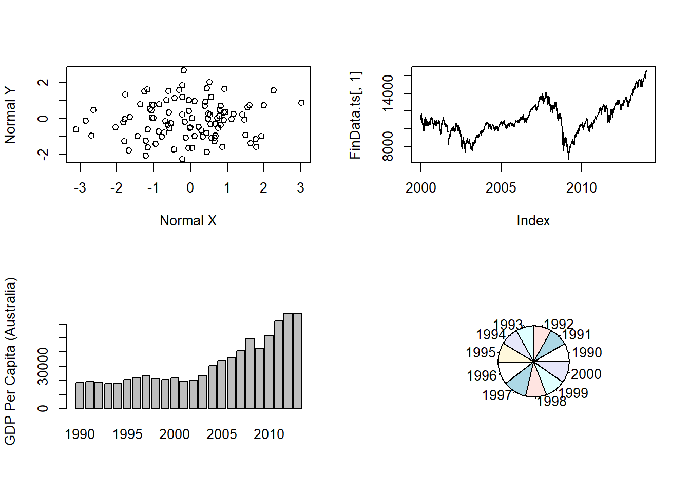
Figure 5.11: Multiple Plots in a Grid
5.3 Introduction to ggplot2
- ggplot2 (Wickham, 2009) is an R package which provides a large variety of plotting functionality to enable better and highly customisable graphs.
- These functions in ggplot2 are based on the grammar of graphics (Wickham, 2010) which is a more formal and structured way to plotting, for a list of various possible graphs, customisation settings and procedures see https://ggplot2.tidyverse.org/
5.3.1 \(\mathtt{qplot}\)
\(\mathtt{qplot}\) stands for quick plot and it makes is easy to produce plots which may often require several lines of codes using base R graphics system.
\(\mathtt{qplot}\) is particularly useful for beginners as they are just getting used to the \(\mathtt{plot}\) function from the base package also the data arguments in \(\mathtt{qplot}\) are same as in the \(\mathtt{plot}\) function (see \(\mathtt{help(qplot)}\) for other arguments to the function).
x = rnorm(100)
y = rnorm(100)
# load the library
library(ggplot2)
# simple scatterplot using qplot
qplot(x, y)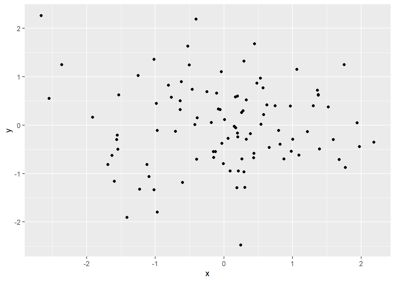
Figure 5.12: Scatterplot using qplot
The argument geom, which stands for geometric objects drawn to represent data has to be changed to “line” create this line plot.
Similarly there is an option to plot histograms using the argument geom=“histogram”
load("data/data_fin.RData")
# line plot using qplot
qplot(x = FinData$Date, y = FinData$DJI, geom = "line", xlab = "Dates", ylab = "Prices",
    main = "DJIA Price Timeseries")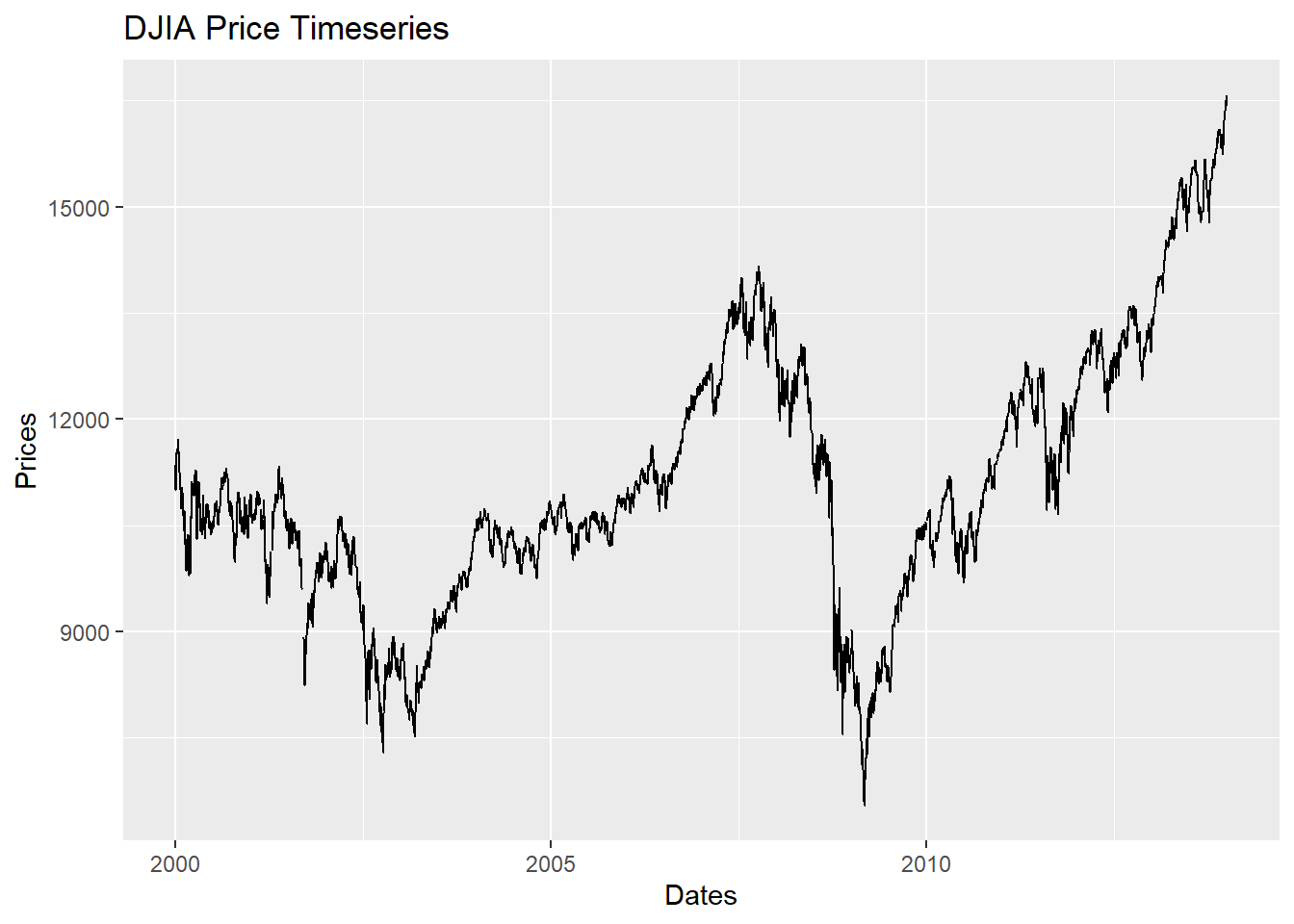
Figure 5.13: Line Plot with lables using qplot
5.3.2 Layered graphics using \(\mathtt{ggplot}\)
The \(\mathtt{qplot}\) function is just sufficient for creating various plots with better presentation compared to base R plots but the true capabilities of ggplot2 are realised by the function \(\mathtt{ggplot}\).
It is important to note that \(\mathtt{ggplot}\) function requires the data in “long” format and hence it is required to first transform the dataset to “long” from “wide” format as in ggplot2, groups are identified by rows, not by columns.
# Read 'long' format data
load("data/GDP_l.RData")
# data snapshot
head(GDP_l)
Year Country GDP
1 1990 Australia 18247.39
2 1991 Australia 18837.19
3 1992 Australia 18599.00
4 1993 Australia 17658.08
5 1994 Australia 18080.70
6 1995 Australia 20375.30# creating the aesthetics using ggplot
p1 = ggplot(GDP_l, aes(Country, GDP, fill = Year))- A plot can be created by adding another layer to p1
# figure
p1 + geom_bar(stat = "identity")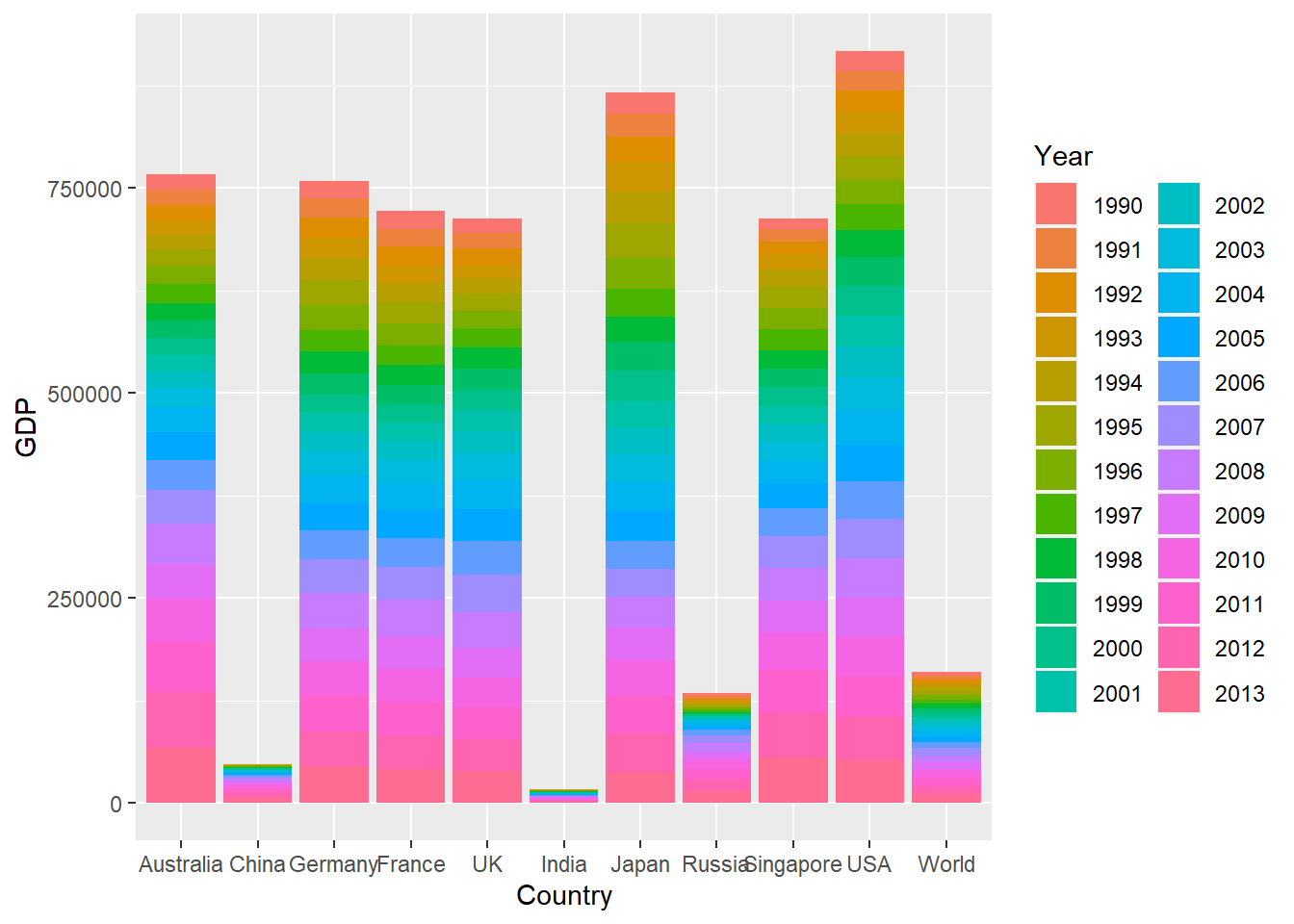
Figure 5.14: Bar Chart Using ggplot function
- To draw a line chart using \(\mathtt{ggplot}\), \(\mathtt{geom\_line()}\)
# change the aesthetics to show time on X-axis and GDP values on Y-axis the
# colour line fill be according to the country
p2 = ggplot(GDP_l, aes(Year, GDP, colour = Country, group = Country))
p2 + geom_line()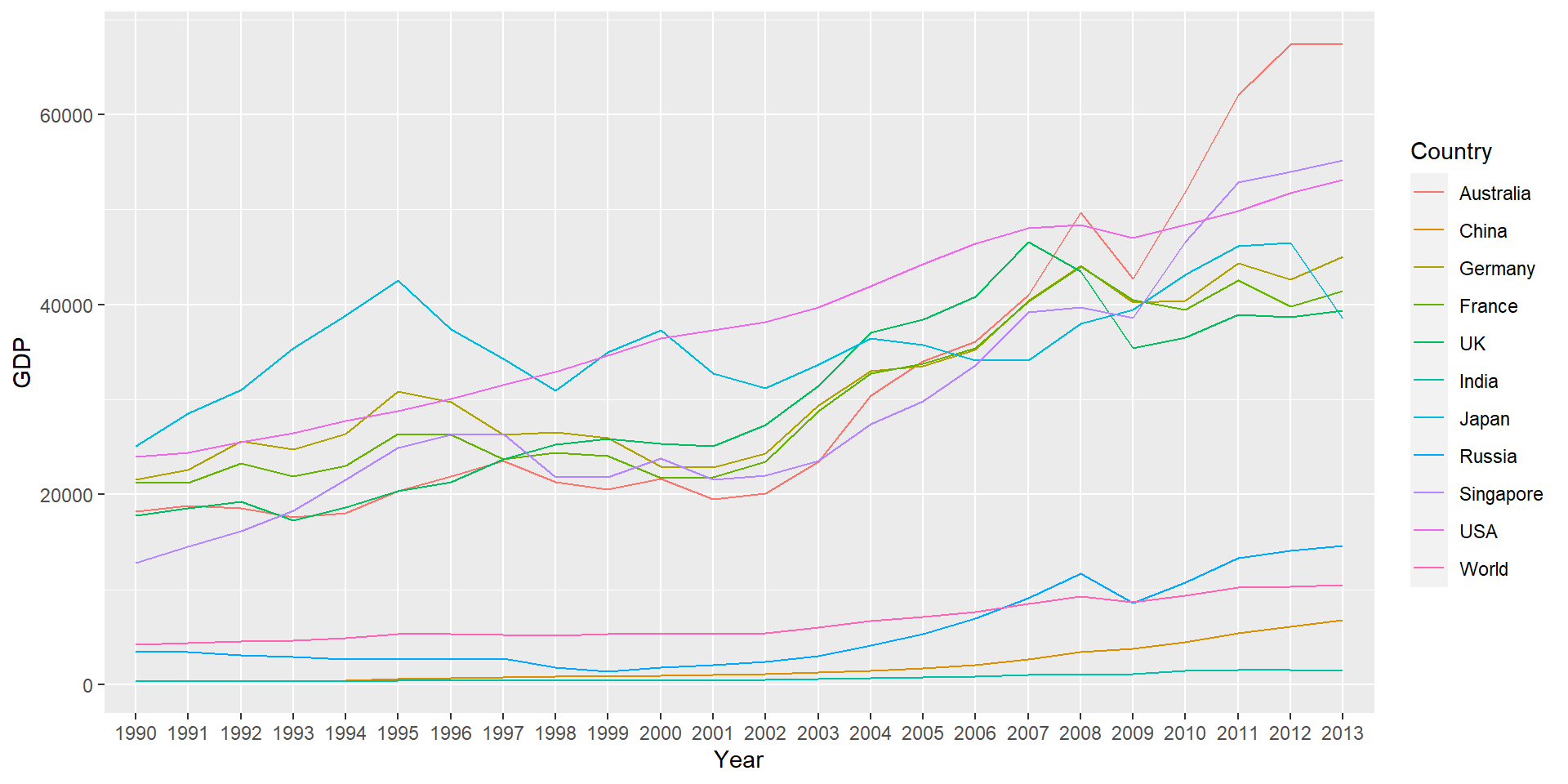
Figure 5.15: Line Chart Using ggplot
These lines can also be drawn in separate panels using faceting. Faceting creates a subplot for each group side by side.
Faceting can be used to either to split the data into vertical groups using \(\mathtt{facet\_grid}\) or horizontal groups using \(\mathtt{facet\_wrap}\).
Figure plots GDP for each country in a separate subplot using grid faceting.
# change the aesthetics to show time on X-axis and GDP values on Y-axis the
# colour line fill be according to the country
p2 = ggplot(GDP_l, aes(Year, GDP, colour = Country, group = Country))
p2 + geom_line() + facet_grid(Country ~ .)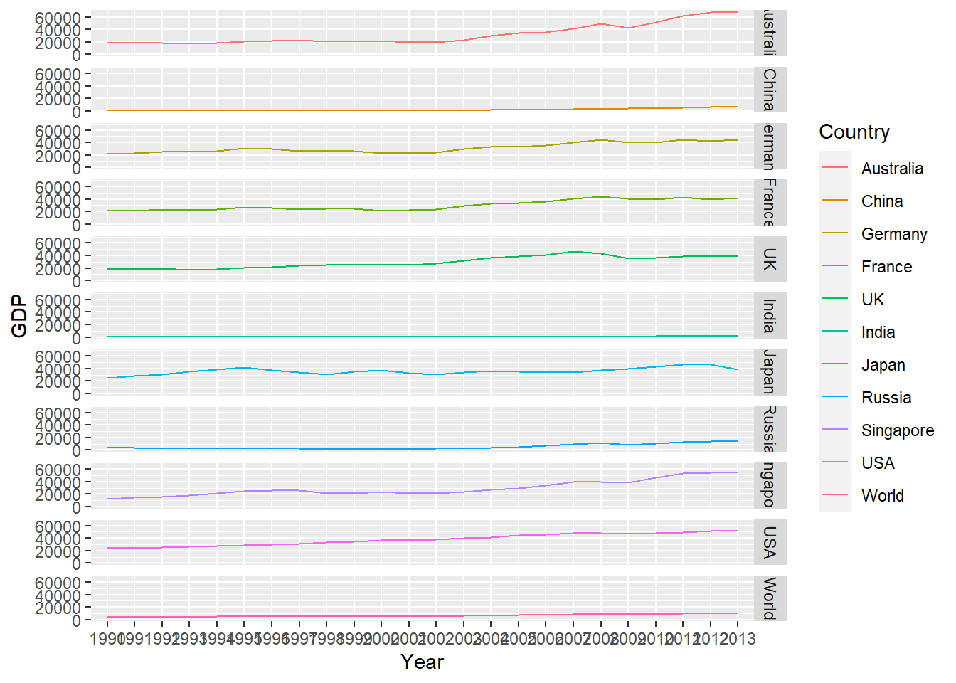
Figure 5.16: Faceting in ggplot (Line Chart)
5.3.3 Arranging plots using gridExtra
There are a few pacakges which allow to arrange ggplots in a grid or a speacific order. gridExtra is one of them and is quite useful in arranging the plots.
Look at the Vignette for egg package for more options. https://cran.r-project.org/web/packages/egg/vignettes/Ecosystem.html
Let’s create three ggplots
p1.1 = ggplot(GDP_l, aes(x = Year, y = GDP))
p2.1 = p1.1 + geom_bar(aes(fill = Country), stat = "identity", position = "dodge")- Stacked bar chart (previous example)
p1.2 = ggplot(GDP_l[GDP_l$Country %in% c("Australia", "UK", "USA"), ], aes(Year,
    GDP))
p2.2 = p1.2 + geom_col(aes(fill = Country)) + labs(title = "GDP for Aus, US and UK")  #using labs to modify title
p2.2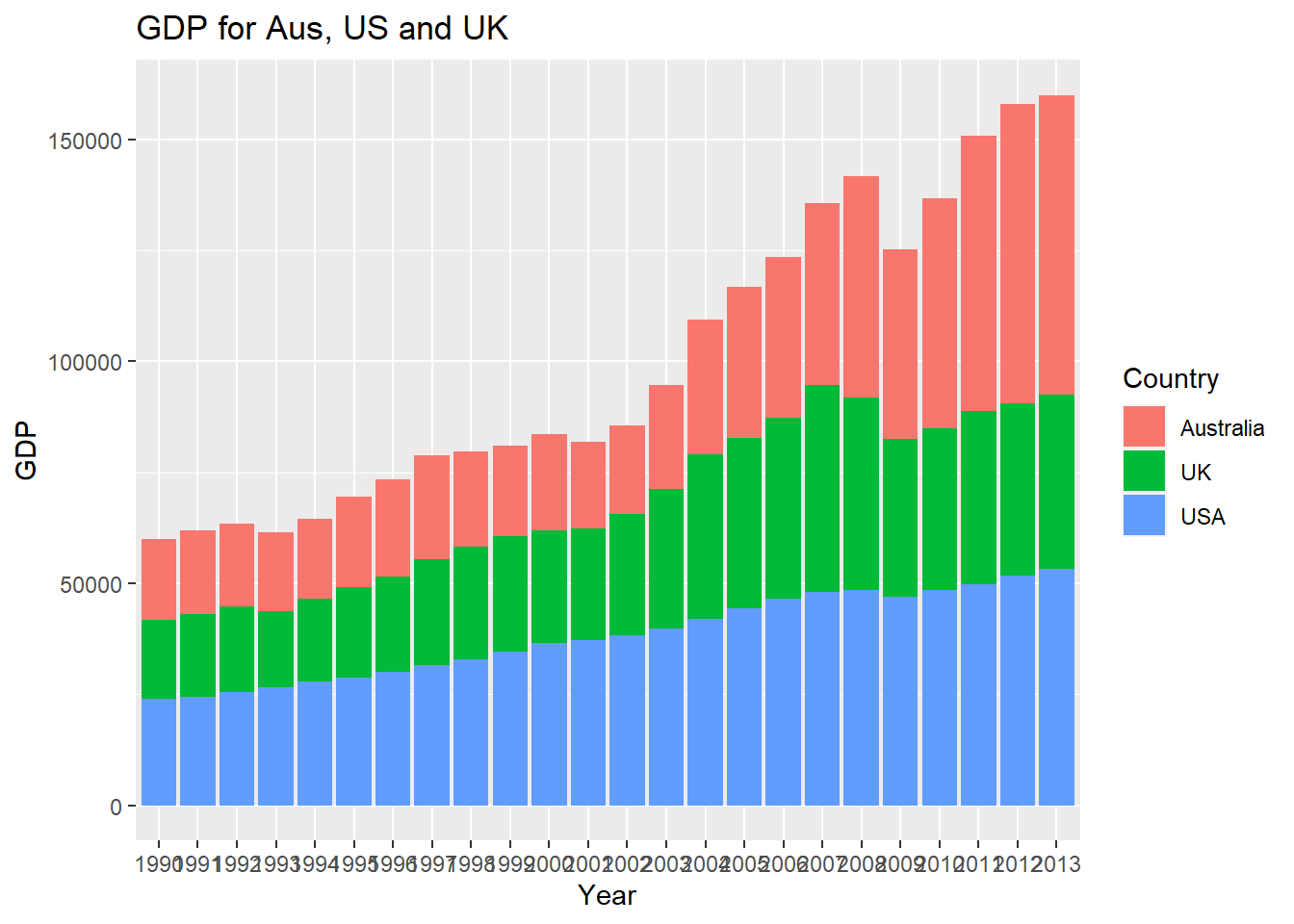
Figure 5.17: Bar Chart with Selected Data
- Stock data
p1.3 = ggplot(FinData, aes(x = Date, y = DJI))
p2.3 = p1.3 + geom_path(colour = "darkblue") + geom_smooth(colour = "black") + theme_linedraw()  #changing theme
p2.3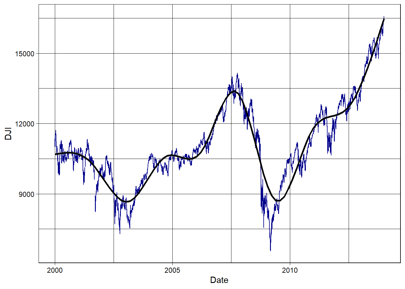
Figure 5.18: Stock Series Plot with Smooth Curve
- Now use gridExtra to put these together
library(gridExtra)
fig1 = grid.arrange(p2.1, p2.2, p2.3, nrow = 3, heights = c(20, 12, 12), top = "Combined plots in three rows")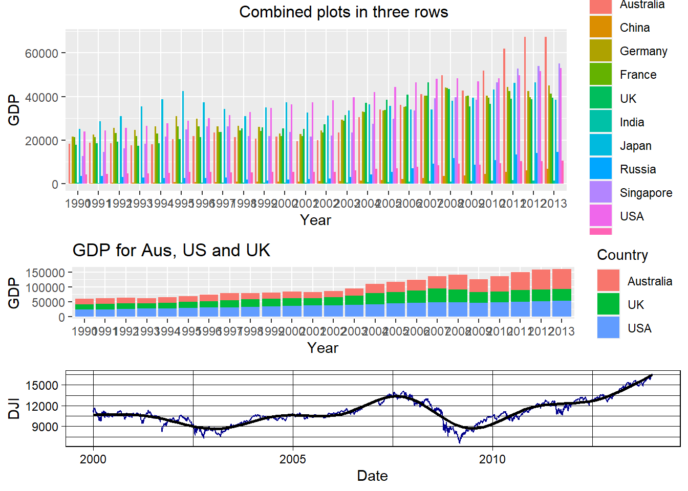
Figure 5.19: Combined plots
- The plots can be saved using the \(\mathtt{ggsave}\) function
ggsave(filename = "combined_plot.pdf", plot = fig1)