Topic 13 Machine Learning using R-Introduction to Data Splitting, Sampling & Resampling

Some references: Boehmke & Greenwell (2019), Hastie, Tibshirani, James, & Witten (2013) and Lantz (2019)
Data science is a superset of Machine learning, data mining, and related subjects. It extensively covers the complete process starting from data loading until production.
“Machine learning is a scientific discipline that is concerned with the design and development of algorithms that allow computers to evolve behaviours based on empirical data, such as from sensor data or databases.” (Wikipedia)
Primary goal of a ML implementation is to develop a general purpose algorithm that solves a practical and focused problem.
Important aspects in the process include data, time, and space requirements.
The goal of a learning algorithm is to produce a result that is a rule and is as accurate as possible.
13.1 Machine Learning Process (Quick Intro)
There are three main phases in an ML process
- Training Phase: Training Data is used to train the model by using expected output with the input. Output is the learning model.
- Validation/Test Phase: Measuring the validity and fit of the model. How good is the model? Uses validation dataset, which can be a subset of the initial dataset.
- Application Phase: Run the model with real world data to generate results
13.2 Data Splitting: Sampling
Training set: data examples that are used to learn or build a classifier.
Validation set: data examples that are verified against the built classifier and can help tune the accuracy of the output.
Testing set: data examples that help assess the performance of the classifier.
Machine Learning requires the data to be split in mainly three categories. The first two (training and validation sets) are usually from the portion of the data selected to build the model on.
Two most common ways of splitting data Overfitting: Building a model that memorizes the training data, and does not generalize well to new data. Generalisation error > Training error.
- Simple random sampling
- Stratified sampling
Typical recommendations for splitting your data into training-test splits include 60% (training)–40% (testing), 70%–30%, or 80%–20%. Its is good to keep the following points in mind:
Spending too much in training (e.g., >80%) won’t allow us to get a good assessment of predictive performance. We may find a model that fits the training data very well, but is not generalizable (overfitting).
Sometimes too much spent in testing (>40% ) won’t allow us to get a good assessment of model parameters.
13.3 Random Sampling
This section explores some ways to conduct random sampling in R. Simple Random sampling does not control for any data attributes.
13.3.1 Base R
The following code uses the BHP close prices to perform a simple random sample using base R sample function.
# import data and select the closing prices
library(xts)  #required as the data was saved as an xts object
d_bhp = readRDS("data/bhp_prices.rds")
d_bhp = d_bhp$BHP.AX.Close  #select close prices
d_bhp = data.frame(Date = as.Date(index(d_bhp)), Price = coredata(d_bhp))  #convert to data frame (for convenience not necessaily required)
head(d_bhp)
Date BHP.AX.Close
1 2019-01-02 33.68
2 2019-01-03 33.68
3 2019-01-04 33.38
4 2019-01-07 34.39
5 2019-01-08 34.43
6 2019-01-09 34.30# use base R function
set.seed(999) #seed is set for reproducibility as the random number generator picks a different seed each time unless specified
idx1 = sample(1:nrow(d_bhp), round(nrow(d_bhp) * 0.7)) #70%
# training set
train1 = d_bhp[idx1, ]
# testing set (remaining data)
test1 = d_bhp[-idx1, ]Note: Sampling is a random process and random number generator produces different results on each execution. Setting a seed in the code keeps it consistent allows for reproducibility.
- Visualise the distribution of training and testing set
library(ggplot2)

p1 = ggplot(train1, aes(x = BHP.AX.Close)) + geom_density(trim = TRUE,
    aes(color = "Training"), size = 1) + geom_density(data = test1, aes(x = BHP.AX.Close,
    color = "Testing"), trim = TRUE, size = 1, linetype = 2)
(p1 = p1 + theme_bw() + labs(color = "Density", title = "Random Sampling (Base R)",
    x = "BHP Prices", y = "Density"))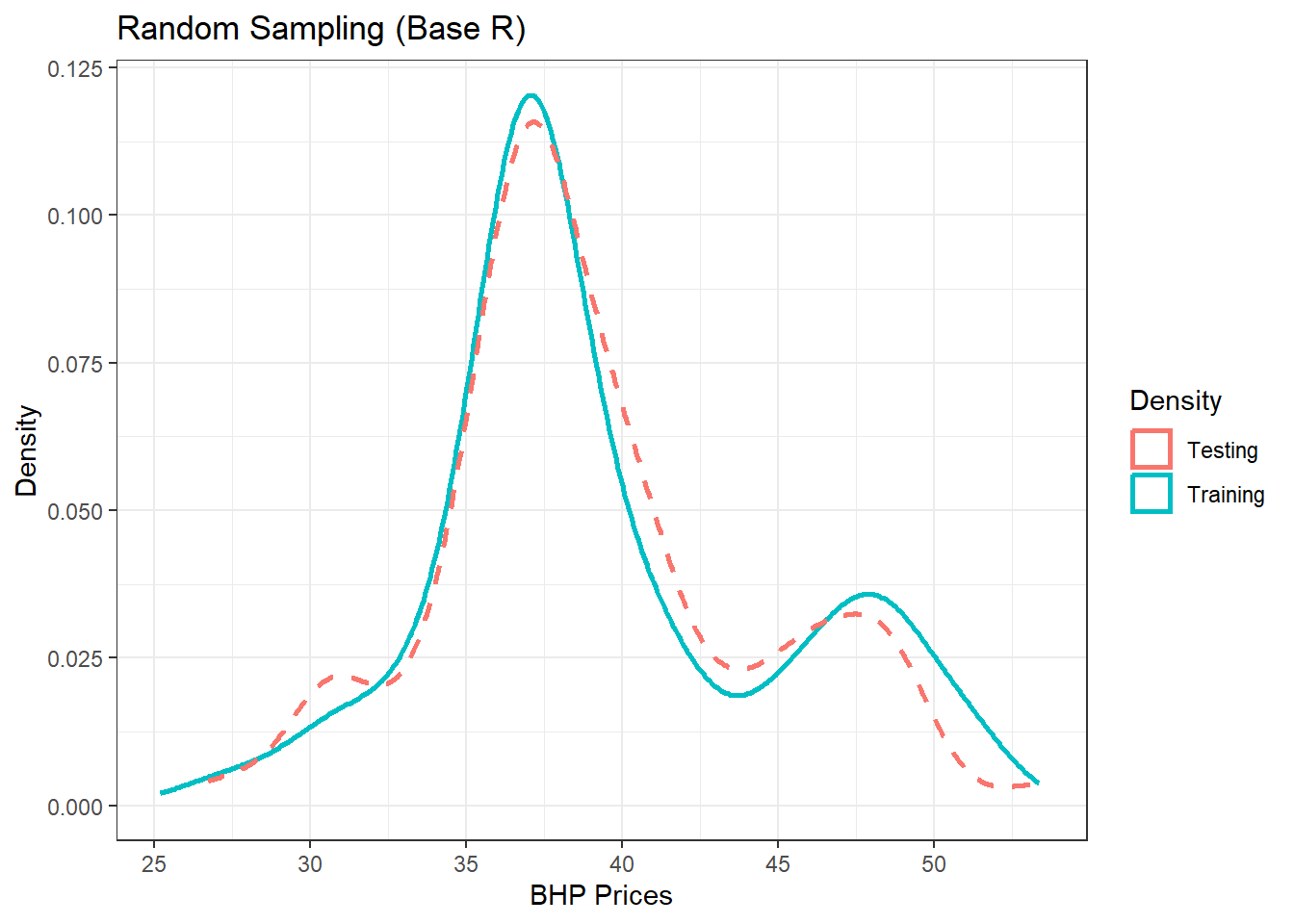
Figure 13.1: Training/Testing using Base R
13.3.2 Using the caret package
- We can use the
caretpackage to create the training and testing samples
set.seed(999)
library(caret)
idx2 = createDataPartition(d_bhp$BHP.AX.Close, p = 0.7, list = FALSE)
train2 = d_bhp[idx2, ]
test2 = d_bhp[-idx2, ]

# plot
p2 = ggplot(train2, aes(x = BHP.AX.Close)) + geom_density(trim = TRUE,
    aes(color = "Training"), size = 1) + geom_density(data = test2, aes(x = BHP.AX.Close,
    color = "Testing"), trim = TRUE, size = 1, linetype = 2)
(p2 = p2 + theme_bw() + labs(color = "Density", title = "Random Sampling (Caret package)",
    x = "BHP Prices", y = "Density"))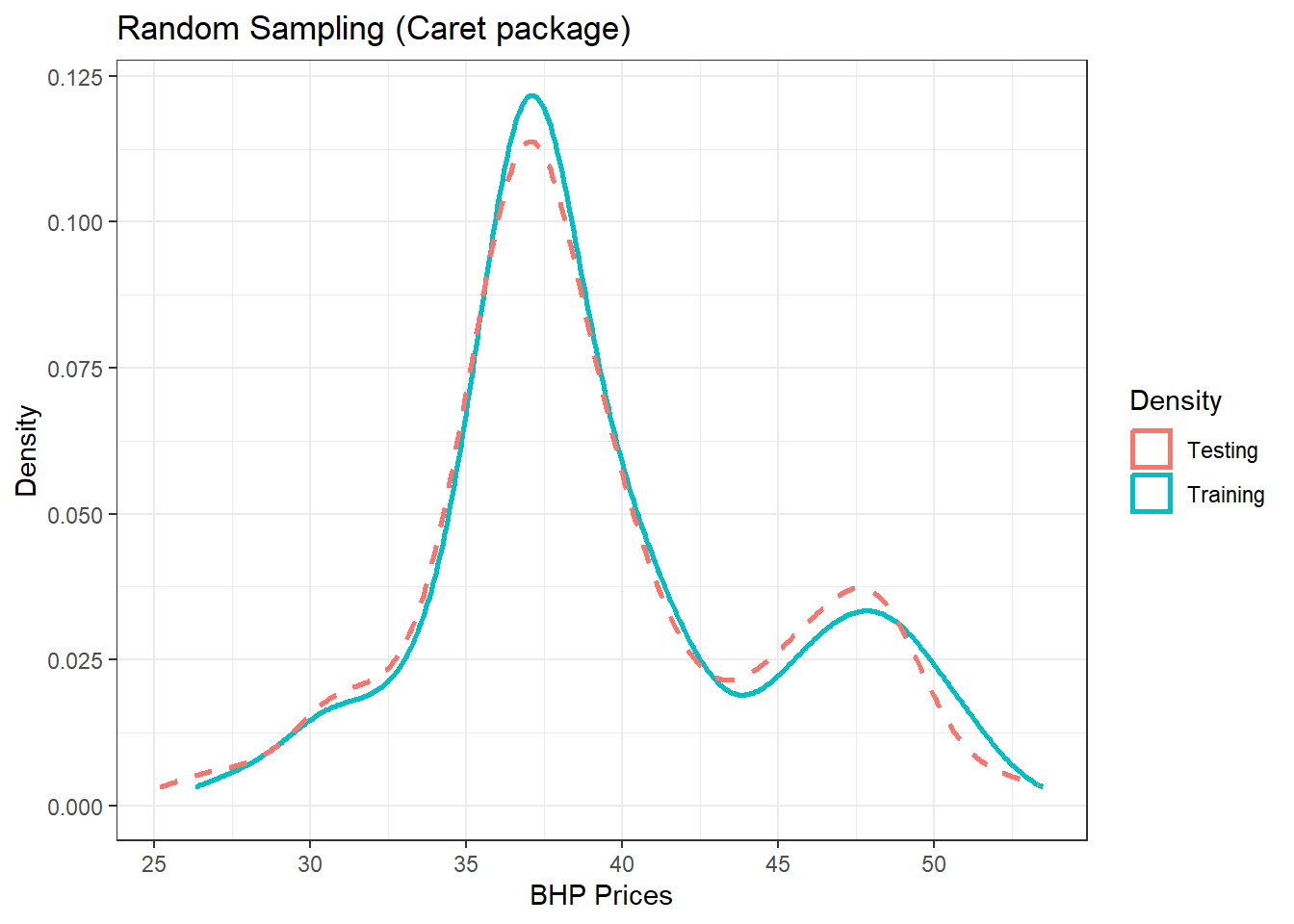
Figure 13.2: Training/Testing using caret
13.3.3 Using the rsample package
- Provides an easy to use method for sampling which is slightly different but can be more convenient due to the function names
set.seed(999)
library(rsample)
idx3 = initial_split(d_bhp, prop = 0.7)  #creates an object to further use for training and testing

train3 = training(idx3)
test3 = testing(idx3)

# plot

p3 = ggplot(train3, aes(x = BHP.AX.Close)) + geom_density(trim = TRUE,
    aes(color = "Training"), size = 1) + geom_density(data = test3, aes(x = BHP.AX.Close,
    color = "Testing"), trim = TRUE, size = 1, linetype = 2)

(p3 = p3 + theme_bw() + labs(color = "Density", title = "Random Sampling (rsample package)",
    x = "BHP Prices", y = "Density"))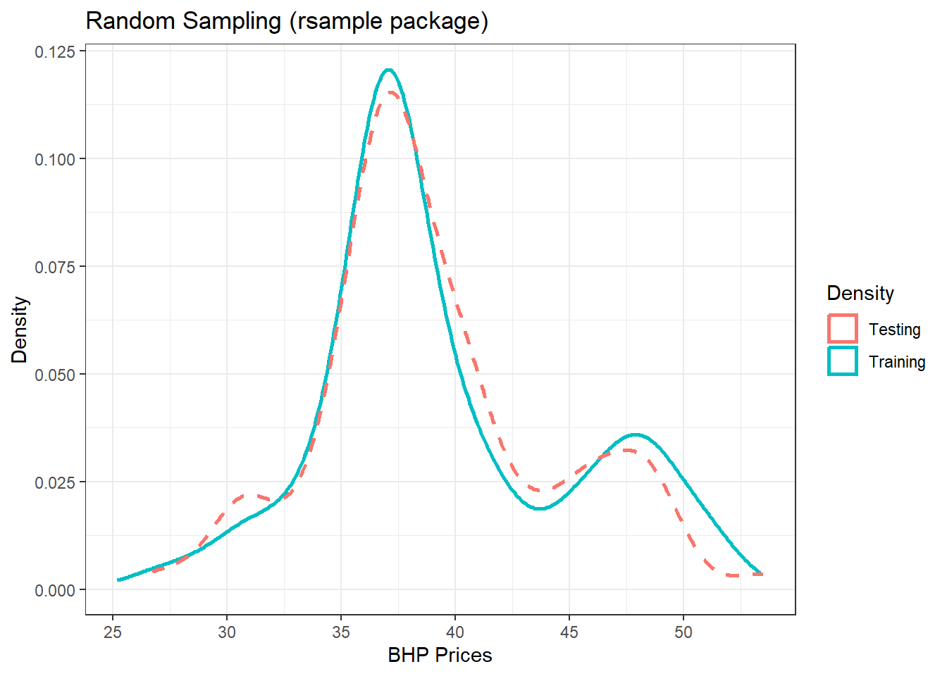
Figure 13.3: Training/Testing using rsample
Combine all three plots
- Notice some differences between the three due to the method used.
library(gridExtra)
grid.arrange(p1, p2, p3, nrow = 1)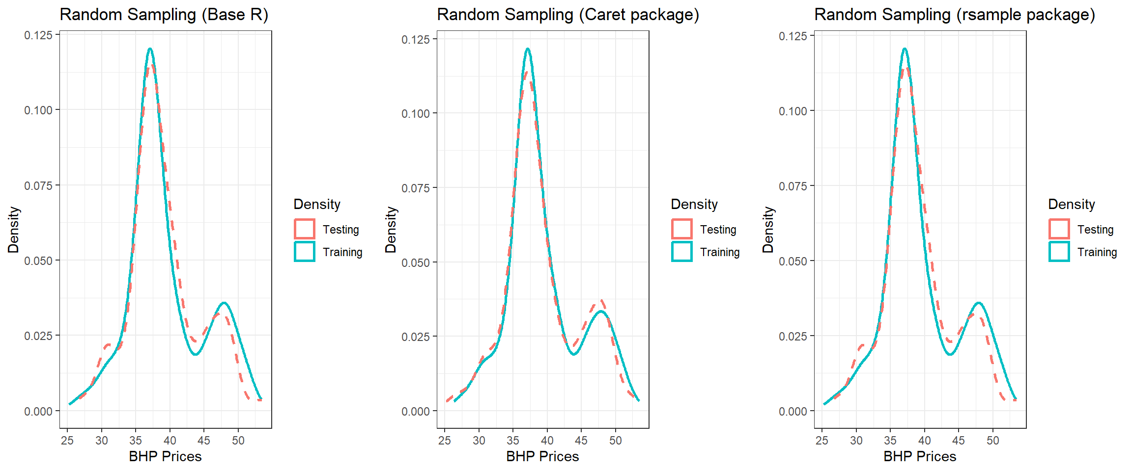
Figure 13.4: Splitting using three methods
13.4 Stratified Sampling
- Random sampling does not control for the proportion of the target variables in the sampling process.
- Machine Learning methods may require similar proportions in the training and testing set to avoid imbalanced response variable.
- Stratified sampling is able to obtain similar distributions for the response variable.
- It can be applied to both, classification or regression problems.
- With a continuous response variable, stratified sampling will segment Y (response variable) into quantiles and randomly sample from each. Consequently, this will help ensure a balanced representation of the response distribution in both the training and test sets.
rsamplepackage can be used to create stratified samples.- The following code demonstrates that on a dataset suitable for classification.
set.seed(999)
data("GermanCredit")  #credit risk data from the caret package
idx4 = initial_split(GermanCredit, prop = 0.7, strata = "Class")  #Class is the binary response variable
train4 = training(idx4)
test4 = testing(idx4)
# check the proportion of outcomes

prop.table(table(train4$Class))  #training set
      Bad      Good
0.3004292 0.6995708 prop.table(table(test4$Class)) #testing set
      Bad      Good
0.2990033 0.7009967
The above training and testing set will have the same proportion of the class values.
13.5 Resampling
The last section demonstrated creation of training and testing dataset for the ML process.
Its not adviced to use the test set to assess model performance during the training phase.
How do we assess the generalization performance of the model?
- One option is to assess an error metric based on the training data. Unfortunately, this leads to biased results as some models can perform very well on the training data but not generalize well to a new data set.
Use a validation approach, which involves splitting the training set further to create two parts: a training set and a validation set (or holdout set).
We can then train our model(s) on the new training set and estimate the performance on the validation set.
Validation using single holdout set can be highly variable and produce unreliable results.
- Solution: Resampling Methods
Resampling Methods: Alternative approach, allowing for repeated model fits to parts of the training data and test it on other parts. Two most commonly used methods are:
K-fold Cross validation
Bootstrapping
Let’s briefly discuss these two.
13.6 K-fold Cross Validation
k-fold cross-validation (aka k-fold CV) is a resampling method that randomly divides the training data into k groups (aka folds) of approximately equal size.
The model is fit on k−1 folds and then the remaining fold is used to compute model performance.
This procedure is repeated k times; each time, a different fold is treated as the validation set.
This process results in k estimates of the generalization error.
The k-fold CV estimate is computed by averaging the k test errors, providing us with an approximation of the error we might expect on unseen data.
K-fold CV in R
rsampleandcaretpackage provide functionality to create k-fold CV
set.seed(999)
# using rsample package
cv1 = vfold_cv(d_bhp[2], v = 10)  #v is the number of folds
cv1  #10 folds
# 10-fold cross-validation
# A tibble: 10 × 2
splits id
<list> <chr>
1 <split [588/66]> Fold01
2 <split [588/66]> Fold02
3 <split [588/66]> Fold03
4 <split [588/66]> Fold04
5 <split [589/65]> Fold05
6 <split [589/65]> Fold06
7 <split [589/65]> Fold07
8 <split [589/65]> Fold08
9 <split [589/65]> Fold09
10 <split [589/65]> Fold10# using caret package
cv2 = createFolds(d_bhp$BHP.AX.Close, k = 10)
cv2$Fold01 #gives indices for 10 folds [1] 28 33 38 42 44 52 71 85 97 119 121 122 125 126 135 160 161 168 191
[20] 194 197 201 222 227 231 239 241 246 265 284 292 298 302 310 319 331 336 344
[39] 353 362 368 384 386 387 402 403 406 430 466 471 484 500 532 533 539 554 567
[58] 570 581 585 610 612 633 641 64213.7 CV for time series data
k-fold cv is random and doesnt preserve the order of the dataset
The order is important in time series applications which are common in financial data science.
One method is to use Time series cross validation. Hyndman & Athanasopoulos (2019) https://otexts.com/fpp3/ section 5.9 provides detailed introduction to the technique.
Basic idea
- The corresponding training set consists only of observations that occurred prior to the observation that forms the test set.
- No future observations can be used in constructing the forecast.
- Since it is not possible to obtain a reliable forecast based on a small training set, the earliest observations are not considered as test sets.
CV for time series in R
- There are several ways to create time series samples in R. The caret package provides a function to accomplish this as well.
- The following creates time slices with a moving window of 500 days (initial window size) with a test period of 100 days (horizon)
- The function returns a list with two elements, train and test with training sample and testing sample
d_bhp2 = xts(d_bhp$BHP.AX.Close, order.by = d_bhp$Date)
cv_ts = createTimeSlices(d_bhp2, initialWindow = 500, horizon = 100, fixedWindow = TRUE)
13.8 Bootstrapping
Bootstrapping is any test or metric that uses random sampling with replacement, and falls under the broader class of resampling methods. Bootstrapping assigns measures of accuracy (bias, variance, confidence intervals, prediction error, etc.) to sample estimates. (Wikipedia)
This means that, after a data point is selected for inclusion in the subset, it’s still available for further selection.
A bootstrap sample is the same size as the original data set from which it was constructed.
Since observations are replicated in bootstrapping, there tends to be less variability in the error measure compared with k-fold CV.
Bootsrapping in R
- rsample package provides
bootstrapsfunction for bootstrapping a sample
boot1 = bootstraps(d_bhp[2], times = 10)
boot1
# Bootstrap sampling
# A tibble: 10 × 2
splits id
<list> <chr>
1 <split [654/241]> Bootstrap01
2 <split [654/253]> Bootstrap02
3 <split [654/240]> Bootstrap03
4 <split [654/226]> Bootstrap04
5 <split [654/223]> Bootstrap05
6 <split [654/242]> Bootstrap06
7 <split [654/241]> Bootstrap07
8 <split [654/240]> Bootstrap08
9 <split [654/258]> Bootstrap09
10 <split [654/249]> Bootstrap10