Topic 12 Portfolio Modelling using R

This topic provides an introduction to using R for Financial Portfolio Modelling. The chapter will discuss using R for creating multi asset Mean-Variance portfolios.
12.1 Portfolio Analysis (Quick Intro)
Investment is a process of maximising wealth.
We want to maximise expected return
We want to minimise the risk
Risk Premium: Difference between returns of a risky asset and risk free asset \(R_{p}-R_{f}\)
Diversification: Process of diversifying risk in a portfolio.
See Chatper-16 from Ruppert (2015) for further details.
12.2 Mean Variance Portfolio: Important concepts
Expected Return
- Expected return for a group of n assets is calculated as
- Portfolio construction should use discrete returns and not logarithmic returns
Risk
- Risk is generally defined as the “dispersion of outcomes around the expected value”
- Variance and Standard Deviation measure dispersion
- The variance of a random variable X is
where
- E(X) is the expected value of a random variable X. This will be financial returns of a security.
- \(p_{i}\) is the probability of the occurrence of \(x_{i}\)
- expression applies to the variance of a single asset where \(x_{i}=r_{i}\)
Covariance of Returns
- One of the measures of association between two (or more) random variables.
- The covariance is positive if the variables tend to move in the same direction, while it is negative if they tend to move in opposite directions.
- Denoted by \(\sigma_{i,j}\) or \(Cov(r_{i},r_{j})\)
Correlation
- Standardised by standard deviation lies between -1 and 1
- Within the context of portfolio analysis, diversification can be defined as combining securities with less than perfectly positively correlated returns.
- In order for the portfolio analyst to construct a diversified portfolio, the analyst must know the correlation coefficients between all securities under consideration.
Portfolio Return
Its a weighted average
\[\begin{equation} R_{p}=\sum_{i=1}^{n}w_{i}r_{i} \tag{12.5} \end{equation}\]Portfolio Risk
Not a simple weighted average, correlation has to be accounted for.
\[\begin{equation} \sigma_{p}^{2}=E[r_{p}-E(r_{p})]^{2} \tag{12.6} \end{equation}\]where \(r_{p}=(w_{1}r_{1}+w_{2}r_{2})\) for a two asset portfolio. After substitution.
\[\begin{equation} \sigma_{p}^{2}=E\{w_{1}r_{1}+w_{2}r_{2}-[w_{1}E(r_{1})+w_{2}E(r_{2})]\}^{2} \tag{12.7} \end{equation}\]After rearranging and expansion
\[\begin{equation} \sigma_{p}^{2}=E\{w_{1}^{2}[r_{1}-E(r_{1})]^{2}+w_{2}^{2}[r_{2}-E(r_{2})]^{2}+2w_{1}w_{2}[r_{1}-E(r_{1})][r_{2}-E(r_{2})]\}\tag{12.8} \end{equation}\] \[\begin{equation} \sigma_{p}^{2}=w_{1}^{2}\sigma_{1}^{2}+w_{2}^{2}\sigma_{2}^{2}+2w_{1}w_{2}\sigma_{12} \tag{12.9} \end{equation}\]where \(\sigma_{12}=Cov(r_{1},r_{2})\)
Portfolio Risk for N Assets
Here we consider 3 assets but the method is generalisable to N assets.
- Matrix of mean returns
- Matrix of weights
\(\sum w=1\)
- Variance-covariance matrix
- Portfolio expected return
- Portfolio variance
See chapter-2 and 3 of Francis & Kim (2013) for further details
12.3 Diversification & Markowitz Minimum Variance Portfolio
Chapter-4 from Szylar (2013) provides an easy to follow introduction and futher details.
Objective: Rational investors; maximise the expected return for a given risk, and they minimise the risk for a given return.
- A minimum variance set is the set of all portfolios that have the least volatility for each level of possible expected return.
- An efficient set (frontier) is the part of the minimum variance frontier that offers the highest expected return for each level of standard deviation.
- Given the level of risk or standard deviation, investors prefer positions with higher expected return and given the expected return, they prefer the positions of lower risk.
- Taking this into account, we can determine the minimum variance set.
- The point where the standard deviation is at its lowest is the global minimum variance portfolio (GMV).
- Portfolios that lie from the GMV portfolio upwards provide investors with the best risk–return combinations and thus are the candidates for the optimal portfolio.
- These portfolios are called the efficient set (frontier); and in order to be on the efficient frontier, the portfolios have to satisfy the following criterion:
- Given a particular level of standard deviation, the portfolios in the efficient set have the highest attainable expected rate of return.
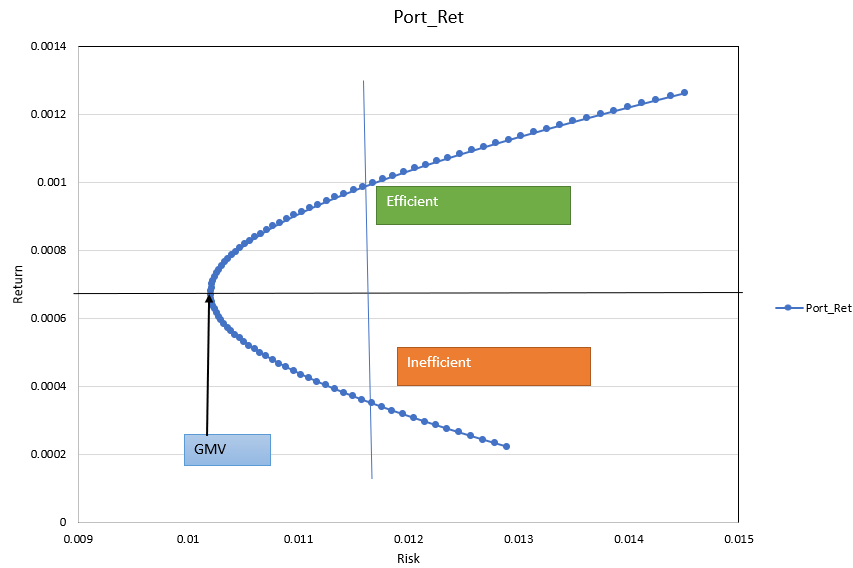
Figure 12.1: Efficient Frontier
12.4 Minimum Variance Portfolio
• A minimum variance (risk) portfolio
\[\begin{equation} Minimise\,\sigma_{p}^{2}=w^{\prime}\Sigma w \tag{12.14} \end{equation}\]subject to
\[\begin{equation} w^{\prime}\mu=\mu_{p} \tag{12.15} \end{equation}\]and
\[\begin{equation} w^{\prime}1=1 \tag{12.16} \end{equation}\]The above constraints apply to long only portfolios. Summation of weights can be different for long and short combination
Portfolio can be formed for a target return and minimum risk or just for minimum risk or with maximum return with minimum risk (mean variance)
With different stocks and asset types, individual weight limits can be imposed.
12.4.1 Efficient Weights for Two Assets
- For a portfolio with Two Risk Assets, the mean variance portfolio weights are calculated as
The above is derived after taking the first derivative of the portfolio variance w.r.t the weight of asset 1,\(w_{1}\). Set that derivative equal to zero and solve for \(w_{1}\).
\[\begin{equation} \frac{\partial\sigma_{p}^{2}}{\partial w_{1}}=\frac{\partial}{\partial w_{1}}\left[w_{1}^{2}\sigma_{1}^{2}+(1-w_{1})^{2}\sigma_{2}^{2}+2w_{1}(1-w_{1})\sigma_{12}\right] \tag{12.19} \end{equation}\]12.4.2 Portfolio with N Risky Assets
Optimisation using Quadratic Programming-Brief overview
To recap: Given a target return \(\mu_{p}\), the efficient portfolio minimises
subject to
\[w^{\prime}\mu=\mu_{p}\]
and
\[w^{\prime}1=1\]
Quadratic Programming is used to minimise a quadratic objective function subject to linear constraints.We focus on the implementation on the technique for optimisation not the mathematical details. Students are expected to learn how to use the method in R
In applications to portfolio optimization, the objective function is the variance of the portfolio return.
The objective function is a function of N variables, such as the weights of N assets, that are denoted by an N × 1 vector x. Suppose that the quadratic objective function to be minimized is
\[\begin{equation} \frac{1}{2}x^{\prime}Dx-d^{\,\prime}x \tag{12.21} \end{equation}\]
where D is an \(N\mathtt{X}N\) matrix and d is an \(N\mathtt{x}1\) vector. The factor of 1/2 is used make the optimisation consistent with R
Two types of linear constraints on x ; inequality and equality
- Inequality constraint
\[A_{neq}^{\prime}x\geq b_{neq}\]
- Equality
\[A_{eq}^{\prime}x=b_{eq}\]
To apply quadratic programming
- \(x=w\)
- \(D=2\Sigma\)
- d is an \(N\mathtt{x}1\) vector of zeros so that (12.21) is \(w^{\prime}\Sigma w\), the return variance of the portfolio.
– R package quadprog has a function called solve.QP to achieve this.
– R package tseries has portfolio.optim function using the solve.QP to make it easier
12.5 Using R to Construct Multi-Asset Portfolio
- This section will contruct a five (5) stock portfolio using prices downloaded from Yahoo finance
- The exercise first creates random weight portfolios then uses two packages PortfolioAnalytics and fPortfolio for risk-return efficient portfolios.
12.5.1 Data
- Download 2 year daily prices for BHP.AX, ANZ.AX, WOW.AX, TLS.AX and CSL.AX
- Stocks are chosen from different sectors
library(quantmod)
library(TTR)
# create a vector of stocks
s1 = c("BHP.AX", "ANZ.AX", "WOW.AX", "TLS.AX", "CSL.AX")

# download prices and create returns from Adjusted Prices
data1 = lapply(s1, FUN = function(x) {
    ROC(Ad(getSymbols(x, from = "2019-07-01", to = "2021-06-30", auto.assign = FALSE)),
        type = "discrete") * 100
})  #%returns

# convert to data frame
ret1 = as.data.frame(do.call(merge, data1))
# change columna names
colnames(ret1) = gsub(".AX.Adjusted", "", colnames(ret1))
# remove the first row of missing values
ret1 = ret1[-1, ]
# add dates column
ret1 = data.frame(Date = as.Date(row.names(ret1)), ret1)
row.names(ret1) = NULL
# save the dataframe (not necessarily required, only for
# reproducibility)
saveRDS(ret1, file = "data/port_ret.Rds")- Plot the data
library(pander)
library(ggplot2)
library(tidyr)
library(ggthemes)
ret1 = readRDS("data/port_ret.Rds")
# overview
pander(head(ret1), split.table = Inf)| Date | BHP | ANZ | WOW | TLS | CSL |
|---|---|---|---|---|---|
| 2019-07-02 | 0.8637 | -1.45 | -0.2726 | -0.5222 | 0.6696 |
| 2019-07-03 | 0.09515 | -0.287 | 2.703 | 1.312 | -0.3486 |
| 2019-07-04 | -0.5466 | 1.331 | 0.7096 | 0 | 1.781 |
| 2019-07-05 | -1.338 | -0.03551 | 0.734 | 0.5181 | 1.596 |
| 2019-07-08 | -1.768 | -0.9591 | -1.137 | -0.7732 | -1.491 |
| 2019-07-09 | 1.159 | -0.6815 | 0.6486 | 0.7792 | -0.5874 |
# convert to long
ret_long = pivot_longer(ret1, cols = -c(Date), values_to = "Return", names_to = "Stock")
# plot

port_p1 = ggplot(ret_long, aes(Date, Return, color = Stock)) + geom_path(stat = "identity") +
    facet_grid(Stock ~ .) + theme_minimal() + labs(x = "Date", y = "Returns")
port_p1  #covid crisis period is evident in the plot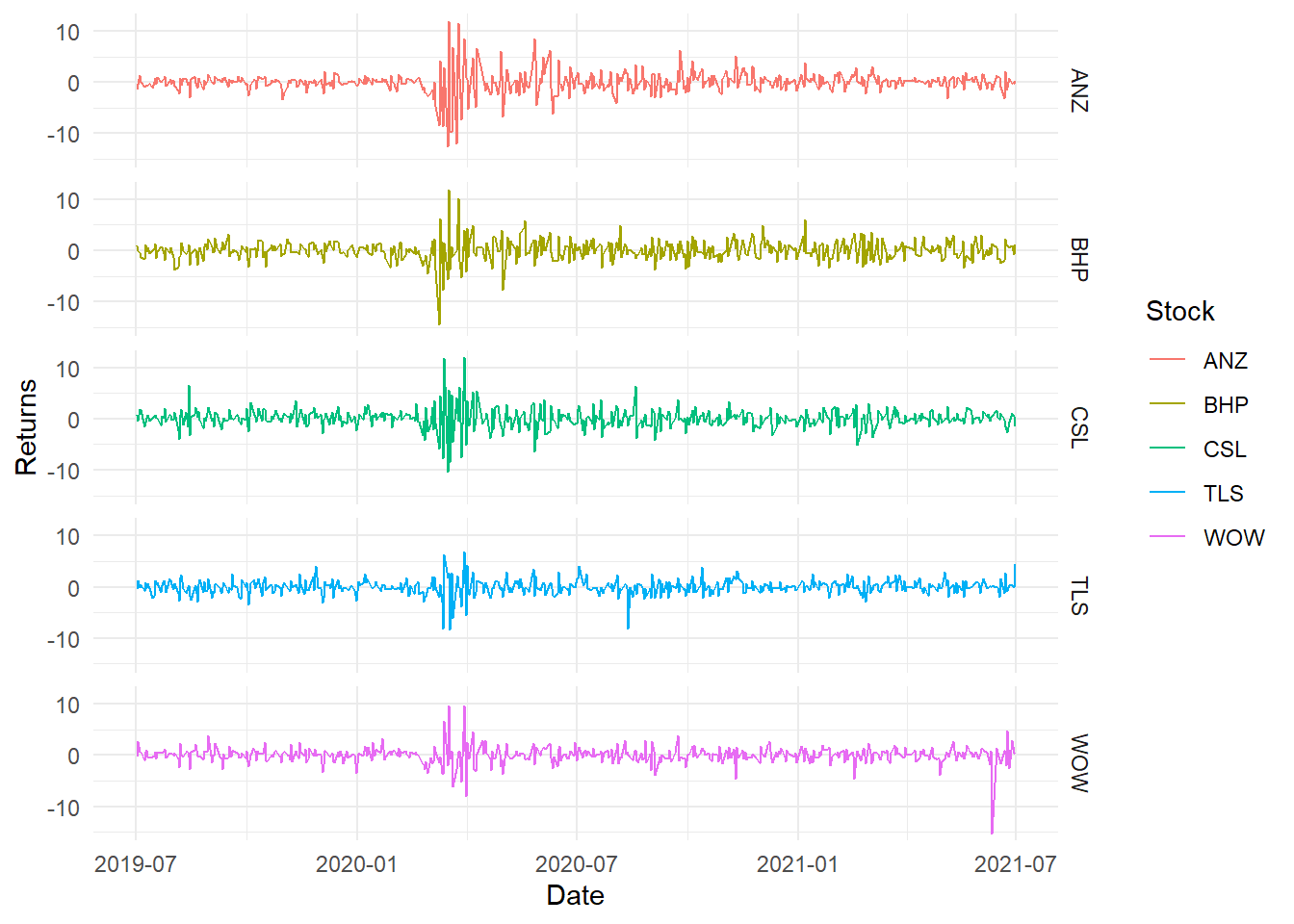
Figure 12.2: Simple returns
12.5.2 Portfolios with random weights
- Calculate the mean returns
- Calculate variance-covariance matrix
- Create series of random weights
- Create series of rerturns and risks
- Create plot
np1 = 200  #number of portfolios
ret2 = ret1[, -1]  #excluding dates
mu1 = colMeans(ret2)  #mean returns
na1 = ncol(ret2)  #number of assets
varc1 = cov(ret2)

riskp1 = NULL  #vector to store risk
retp1 = NULL  #vector to store returns
# using loops here (not aiming for efficiency but demonstration)

for (i in 1:np1) {
    w = diff(c(0, sort(runif(na1 - 1)), 1))  # random weights
    r1 = t(w) %*% mu1  #matrix multiplication
    sd1 = t(w) %*% varc1 %*% w
    retp1 = rbind(retp1, r1)
    riskp1 = rbind(riskp1, sd1)
}

# create a data frame of risk and return
d_p1 = data.frame(Ret = retp1, Risk = riskp1)
# simple plot
plot(d_p1$Risk, d_p1$Ret, xlab = "Risk", ylab = "Return", main = "Frontier Portfolios",
    col = "blue")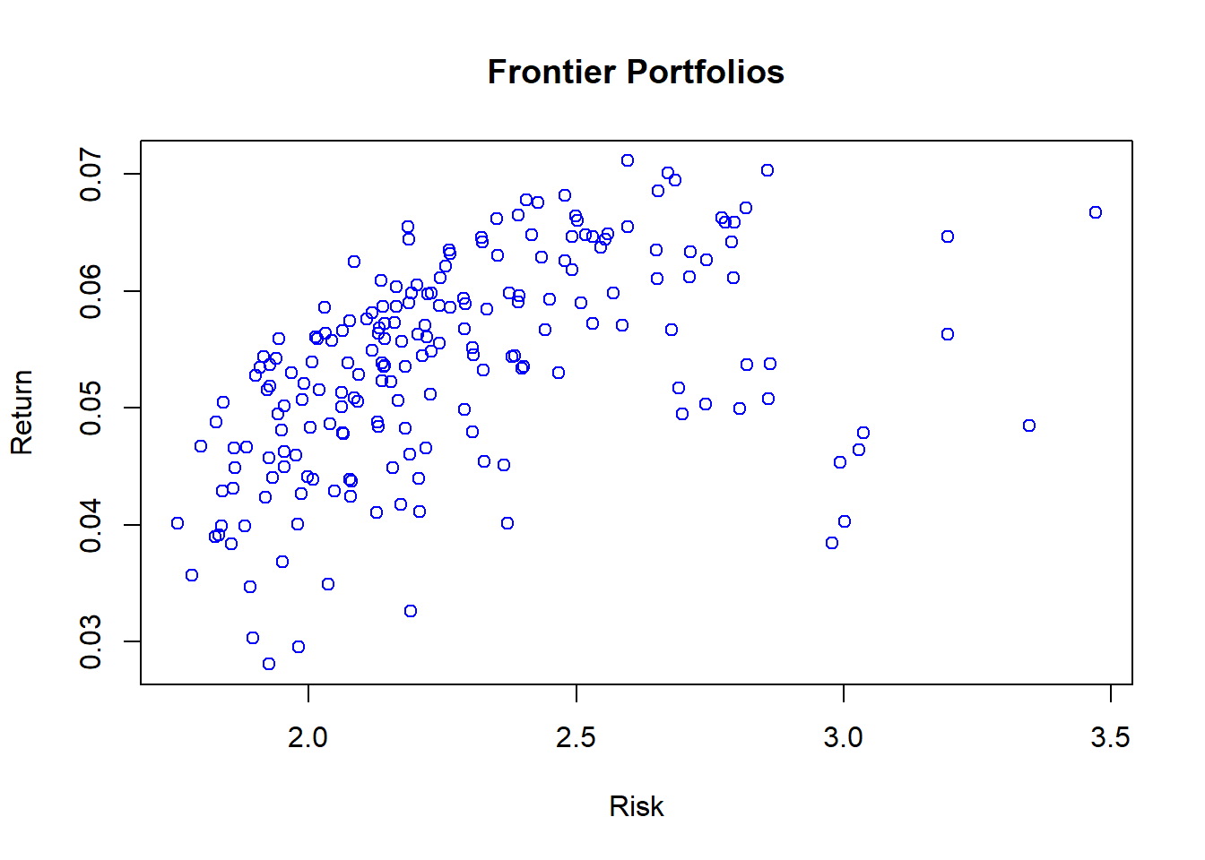
Figure 12.3: Random Portfolios
- Use ggplot2
library(ggplot2)
# first layer
p1 = ggplot(d_p1, aes(Risk, Ret, colour = Ret))
# scatter plot
p1 = p1 + geom_point()
# scatter plot with density and identified port risk return (highest
# lowest returns and min risk)
p1 + geom_point() + geom_hline(yintercept = c(max(d_p1$Ret), median(d_p1$Ret),
    min(d_p1$Ret)), colour = c("darkgreen", "darkgray", "darkred"), size = 1) +
    geom_vline(xintercept = d_p1[(d_p1$Risk == min(d_p1$Risk)), ][, 2]) +
    labs(colour = "Portfolio Return", x = "Portfolio Risk", y = "Portfolio Return",
        title = "Random Feasible Portfolios") + theme_bw()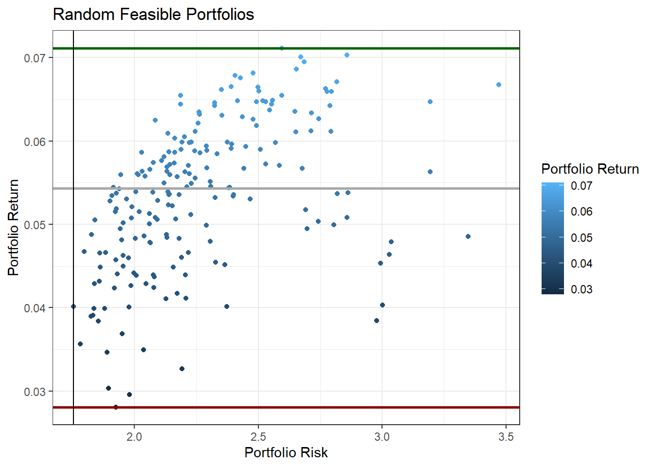
Figure 12.4: Random Portfolios
12.6 Efficient (Minimum Variance) Portfolio using R packages
- R’s PortfolioAnalytics package provides various tools for portfolio anlaytics including minimum variance portfolio optimisation
- Create random portfolios based on risk (Std. Dev.) and reward (mean return)
- Full investment: Allocate in all the assets (minimum 0 and maximum 1 weight)
- Long only: Only buy, no short position (positive weights only)
library(PortfolioAnalytics)
# initialise with asset names uses time series data
data_p2 = zoo(ret1[, -1], order.by = as.Date(ret1$Date))
# create specification
port = portfolio.spec(assets = c(colnames(data_p2)))
# add long only constraint
port = add.constraint(portfolio = port, type = "long_only")
# add full investment contraint
port = add.constraint(portfolio = port, type = "full_investment")

# objective: manimise risk
port_rnd = add.objective(portfolio = port, type = "risk", name = "StdDev")

# objective: maximise return
port_rnd = add.objective(portfolio = port_rnd, type = "return", name = "mean")

# 1. optimise random portfolios

rand_p = optimize.portfolio(R = data_p2, portfolio = port_rnd, optimize_method = "random",
    trace = TRUE, search_size = 1000)
# plot

chart.RiskReward(rand_p, risk.col = "StdDev", return.col = "mean", chart.assets = TRUE)  #also plots the equally weighted portfolio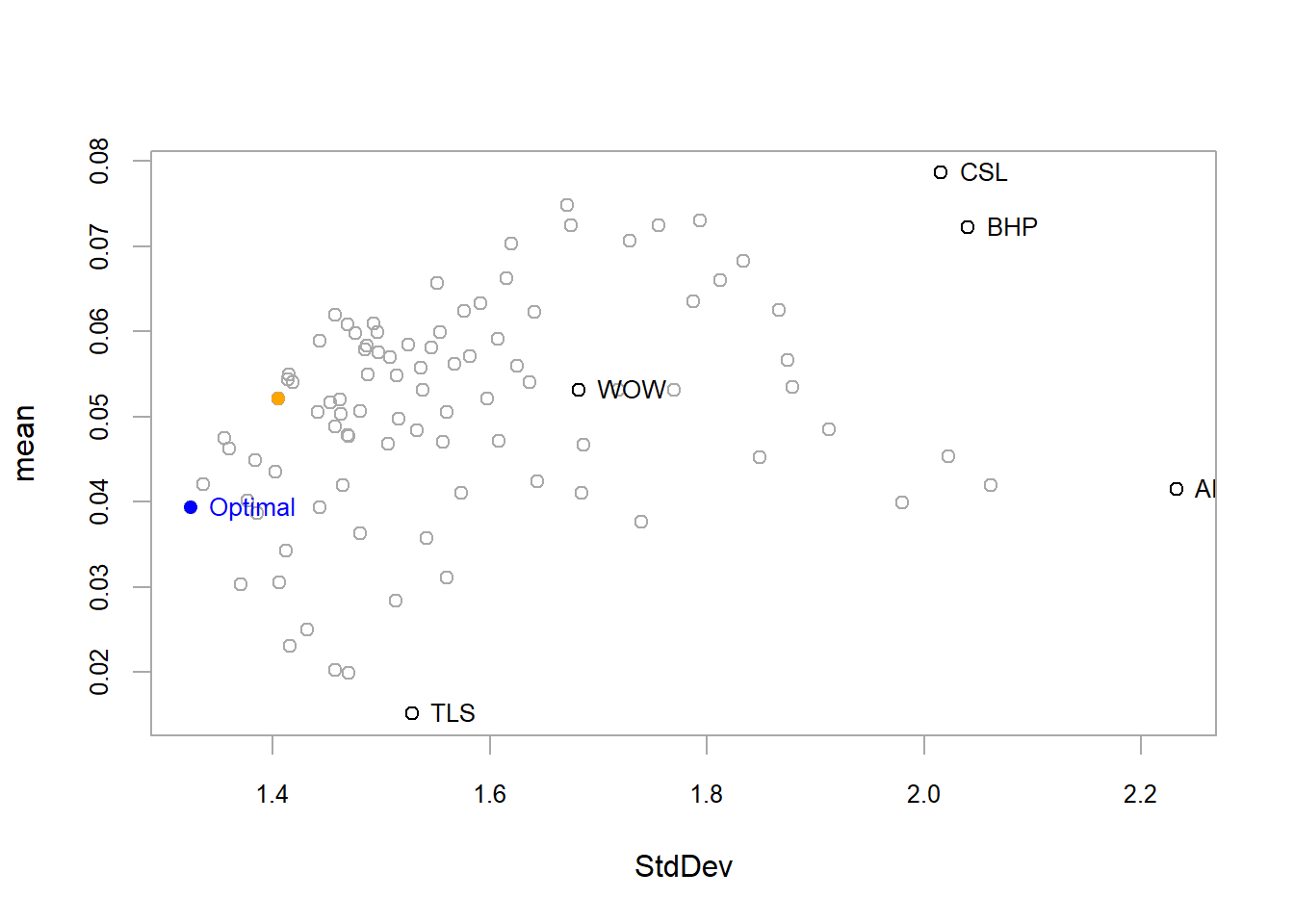
Figure 12.5: Mean-Variance Portfolios
- Optimise for minimum risk
- Minimise the level of Standard Deviation for the portfolio
port_msd = add.objective(portfolio = port, type = "risk", name = "StdDev")
minvar1 = optimize.portfolio(R = data_p2, portfolio = port_msd, optimize_method = "ROI",
    trace = TRUE)
minvar1
***********************************
PortfolioAnalytics Optimization
***********************************
Call:
optimize.portfolio(R = data_p2, portfolio = port_msd, optimize_method = "ROI",
trace = TRUE)
Optimal Weights:
BHP ANZ WOW TLS CSL
0.1437 0.0735 0.3122 0.4543 0.0164
Objective Measure:
StdDev
1.32 # plot
plot(minvar1, risk.col = "StdDev", main = "Mean Variance Portfolio", chart.assets = TRUE)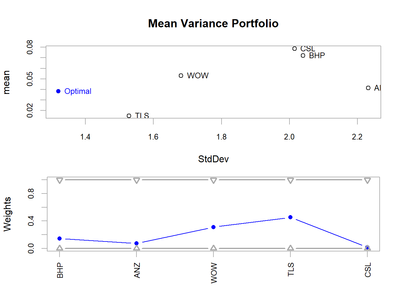
Figure 12.6: Mean Variance Portfolio Risk/Return
# efficient frontier
minvar_ef = create.EfficientFrontier(R = data_p2, portfolio = port_msd,
    type = "mean-StdDev")
chart.EfficientFrontier(minvar_ef, match.col = "StdDev", type = "l", tangent.line = FALSE,
    chart.assets = TRUE)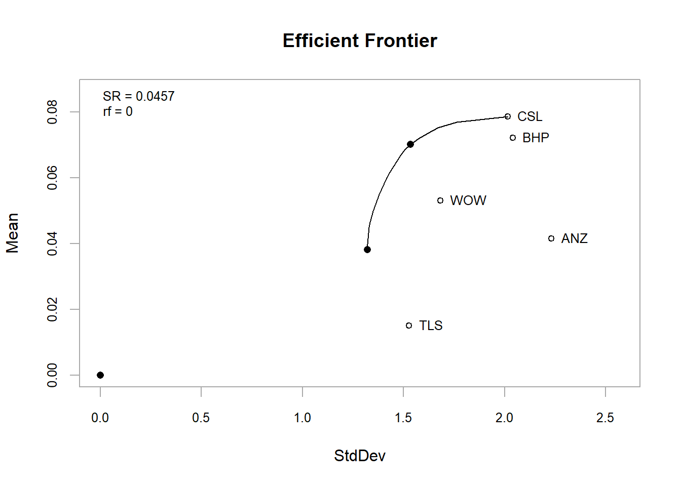
Figure 12.7: Efficient Frontier
- The fPortfolio package also provides functions to conduct the optimisation
- An ebook is available with further details on the fPortfolio package see here https://www.rmetrics.org/ebooks-portfolio
library(fPortfolio)
data_p2 = as.timeSeries(data_p2)
pspec = portfolioSpec()  #initial specification

setNFrontierPoints(pspec) = 500  #random portfolios for the efficient frontier

eff_front2 = portfolioFrontier(data_p2, constraints = "LongOnly")  #strategy
plot(eff_front2, c(1, 2, 4, 5, 6))
Figure 12.8: Efficient frontier plot (fPortfolio)
- Another function (allows to add different points and lines from other portfolios)
- Also plots of the weights in different portfolios
tailoredFrontierPlot(eff_front2, sharpeRatio = FALSE, risk = "Sigma")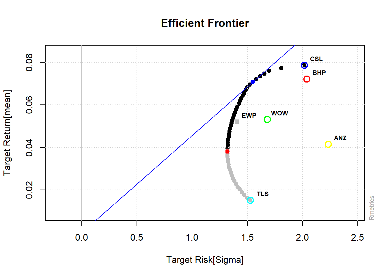
Figure 12.9: Efficient Frontier
# weights
weightsPlot(eff_front2)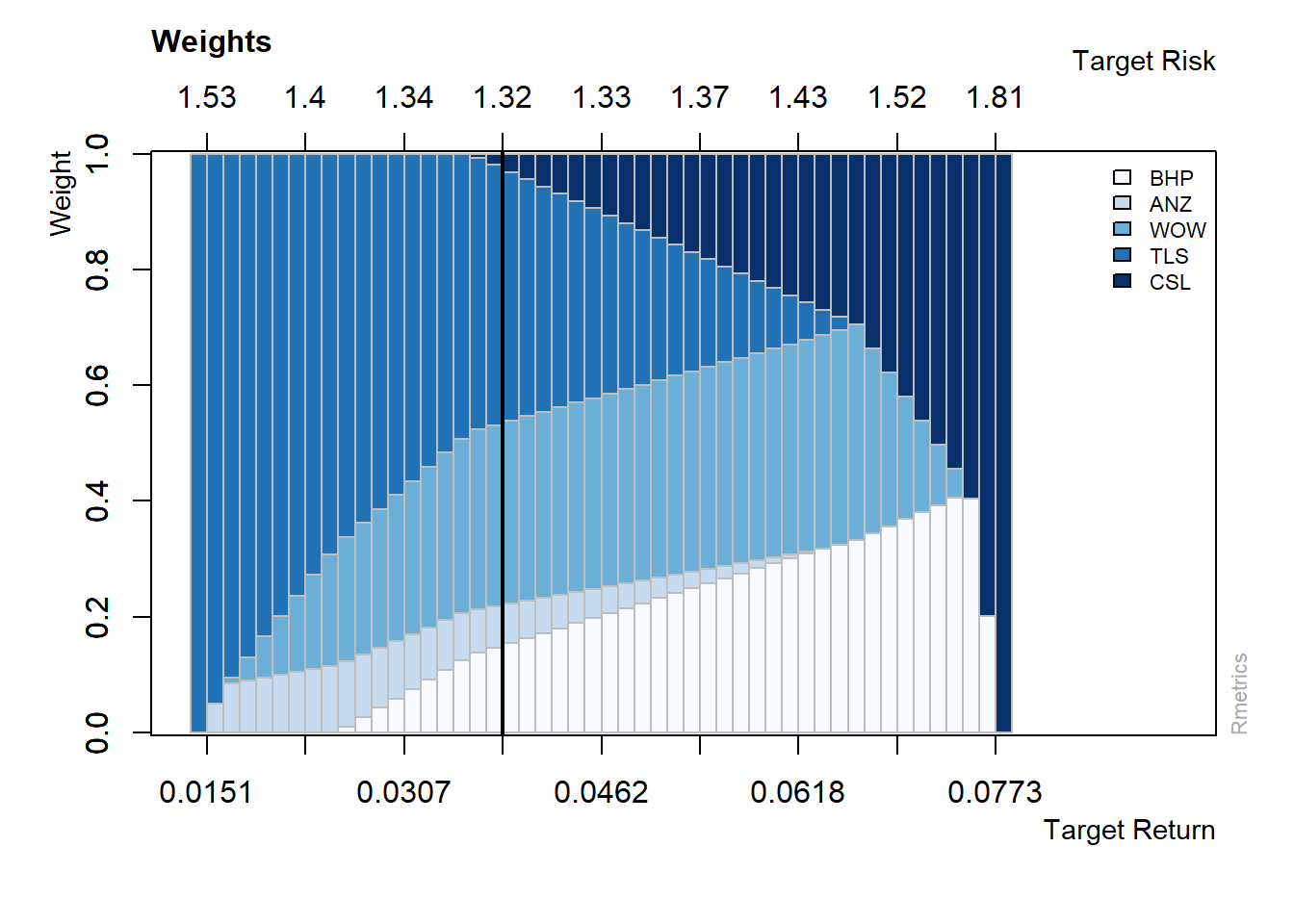
Figure 12.10: Weights Plot
12.6.1 Minimum Variance and portfolio for a given level of return
- Minimum variance
- Uses previous constraints (Long Only)
(minvar2 = minvariancePortfolio(data_p2))
Title:
 MV Minimum Variance Portfolio
 Estimator:         covEstimator
 Solver:            solveRquadprog
 Optimize:          minRisk
 Constraints:       LongOnly

Portfolio Weights:
   BHP    ANZ    WOW    TLS    CSL
0.1437 0.0735 0.3122 0.4543 0.0164

Covariance Risk Budgets:
   BHP    ANZ    WOW    TLS    CSL
0.1437 0.0735 0.3122 0.4543 0.0164

Target Returns and Risks:
  mean    Cov   CVaR    VaR
0.0382 1.3204 3.2805 2.0550

Description:
Wed Dec 7 08:34:42 2022 by user: RMachine - Target Return
mu = mean(colMeans(data_p2))  #target return
setTargetReturn(pspec) = mu
(eff_port2 = efficientPortfolio(data_p2, pspec))
Title:
 MV Efficient Portfolio
 Estimator:         covEstimator
 Solver:            solveRquadprog
 Optimize:          minRisk
 Constraints:       LongOnly

Portfolio Weights:
   BHP    ANZ    WOW    TLS    CSL
0.2364 0.0342 0.3425 0.2360 0.1510

Covariance Risk Budgets:
   BHP    ANZ    WOW    TLS    CSL
0.2563 0.0326 0.3439 0.1994 0.1677

Target Returns and Risks:
  mean    Cov   CVaR    VaR
0.0521 1.3608 3.4011 1.9698

Description:
 Wed Dec  7 08:34:42 2022 by user: RMachine
12.6.2 Portfolio with Box Constraints
- We can add box constraints to setup minimum weights so that we invest in each stock in the portfolio.
- This can be achieved using both packages.
- Here we demonstrate using the fPortfolio package. See help(box_constraints) for PortfolioAnalytics package
pspec2 = portfolioSpec()

setNFrontierPoints(pspec) = 500
boxconstraints = c("minW[1:5]=0.1", "maxW[1:5]=1")  #for minimum asset weights and maximum asset weights
eff_front3 = portfolioFrontier(data_p2, spec = pspec2, constraints = boxconstraints)
eff_front3
Title:
 MV Portfolio Frontier
 Estimator:         covEstimator
 Solver:            solveRquadprog
 Optimize:          minRisk
 Constraints:       minW maxW
 Portfolio Points:  5 of 24

Portfolio Weights:
      BHP    ANZ    WOW    TLS    CSL
1  0.1000 0.1000 0.1248 0.5752 0.1000
6  0.1160 0.1000 0.2713 0.4127 0.1000
12 0.1900 0.1000 0.3253 0.2611 0.1236
18 0.2323 0.1000 0.3382 0.1292 0.2003
24 0.2558 0.1000 0.1000 0.1000 0.4442

Covariance Risk Budgets:
      BHP    ANZ    WOW    TLS    CSL
1  0.0922 0.0983 0.1022 0.6022 0.1052
6  0.1136 0.1040 0.2662 0.4063 0.1099
12 0.2038 0.1069 0.3268 0.2270 0.1354
18 0.2495 0.1038 0.3270 0.0972 0.2225
24 0.2495 0.0917 0.0711 0.0669 0.5209

Target Returns and Risks:
     mean    Cov   CVaR    VaR
1  0.0346 1.3525 3.2604 2.0459
6  0.0410 1.3280 3.3011 2.0827
12 0.0488 1.3482 3.3697 1.9793
18 0.0566 1.3977 3.4827 2.0566
24 0.0644 1.5223 3.7541 2.2943

Description:
Wed Dec 7 08:34:42 2022 by user: RMachine plot(eff_front2, c(1, 2, 4, 5, 6))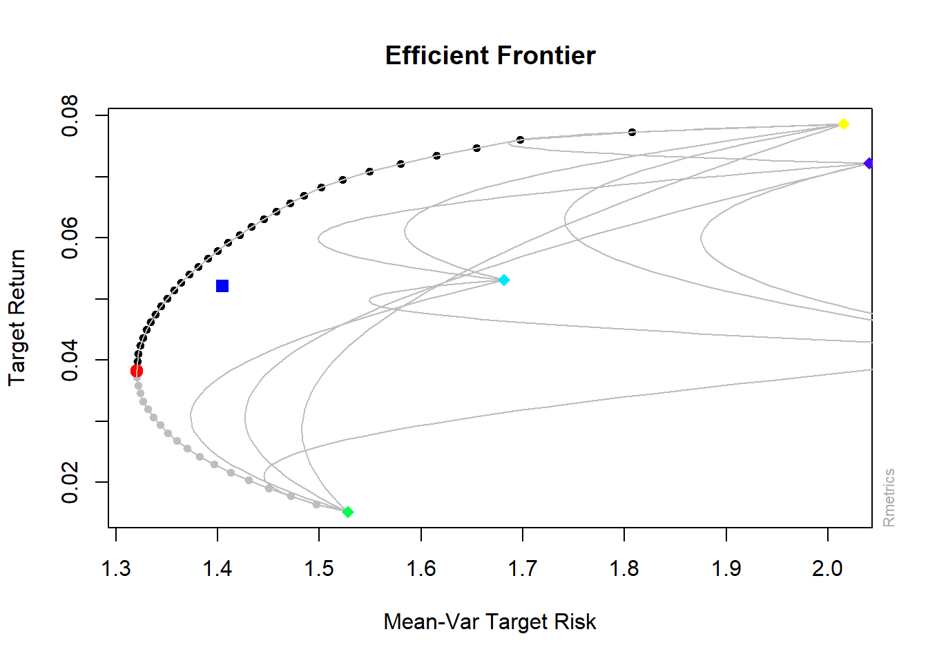
Figure 12.11: Frontier Plot (box constraints)
(minvar3 = minvariancePortfolio(data = data_p2, spec = pspec2, constraints = boxconstraints))
Title:
 MV Minimum Variance Portfolio
 Estimator:         covEstimator
 Solver:            solveRquadprog
 Optimize:          minRisk
 Constraints:       minW maxW

Portfolio Weights:
   BHP    ANZ    WOW    TLS    CSL
0.1179 0.1000 0.2728 0.4093 0.1000

Covariance Risk Budgets:
   BHP    ANZ    WOW    TLS    CSL
0.1158 0.1041 0.2680 0.4021 0.1099

Target Returns and Risks:
  mean    Cov   CVaR    VaR
0.0412 1.3280 3.3025 2.0801

Description:
 Wed Dec  7 08:34:44 2022 by user: RMachine
12.7 Evaluating Portfoios: Risk Adjusted Performance
12.7.2 Roy’s Safety Ratio
Roy’s Safety First (SF) Ratio makes a slight modification to the Sharpe Ratio.
Specifically, instead of using the risk-free rate, Roy’s SF Ratio instead uses a target or minimum acceptable return to calculate the excess return
12.7.3 Treynor’s Ratio
- The Treynor Ratio modifies the denominator in the Sharpe Ratio to use beta instead of standard deviation in the denominator. That is
12.7.4 Sharpe Ratio (Portfolio) in R
- Assume an rf=0.02
- The code uses the fPortfolio package
- The ratio can also be easily calculated using base R
# create specification
pspec3 = portfolioSpec()
setRiskFreeRate(pspec3) = 0.02
setNFrontierPoints(pspec3) = 50
# create efficient frontier
eff_front4 = portfolioFrontier(data_p2, spec = pspec3, constraints = "LongOnly")

# find the tangency port
tgport1 = tangencyPortfolio(data = data_p2, spec = pspec3, constraints = "LongOnly")
# create frontier plot


frontierPlot(eff_front4, pch = 1, auto = FALSE, xlim = c(0, 2.5), ylim = c(0,
    0.085))  #custom x and y limits
minvariancePoints(object = eff_front4, auto = FALSE, col = "red", pch = 20)  #add min variance port
tangencyPoints(object = eff_front4, col = "blue", pch = 20)  #add tangency port
tangencyLines(object = tgport1, col = "darkblue")  #add tangency portfolio line
grid()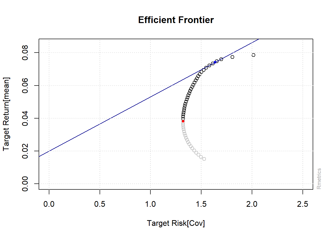
Figure 12.12: Tangency Portfolio (Sharpe Portfolio)
print(tgport1)
Title:
 MV Tangency Portfolio
 Estimator:         covEstimator
 Solver:            solveRquadprog
 Optimize:          minRisk
 Constraints:       LongOnly

Portfolio Weights:
   BHP    ANZ    WOW    TLS    CSL
0.3996 0.0000 0.0758 0.0000 0.5247

Covariance Risk Budgets:
   BHP    ANZ    WOW    TLS    CSL
0.3853 0.0000 0.0464 0.0000 0.5683

Target Returns and Risks:
  mean    Cov   CVaR    VaR
0.0741 1.6352 4.0740 2.4228

Description:
 Wed Dec  7 08:34:44 2022 by user: RMachine
# weights plot weightsPie(tgport1,box=FALSE)
# weightedReturnsPie(tgport1,box=FALSE)