Topic 14 Logistic Regression & K-Nearest Neighbour (kNN) for Classification

This topic provides a brief introduction to two ML methods used for classification; Logistic Regression and K-Nearest Neighbour. The topic includes an example on predicting the direction of stock price movement to illustrate the application of R for these two models.

14.1 Logistic Regression

Logistic Regression belongs to the class of generalised linear models (glms)generalised linear models (glms)
Used to model data with a dichotomous response variable.
Logistic regression models the conditional probability of the response variable rather than its value.
A logit link function, defined as \(logit\,p=log[p/(1-p)]\), is used to transform the output of a linear regression to be suitable for probabilities.
A linear model for these transformed probabilities can be setup as

\[\begin{equation} logit\,p=\beta_{0}+\beta_{1}x_{1}+\beta_{2}x_{2}+\ldots\beta_{k}x_{x} \tag{14.1} \end{equation}\]

R provides the glm function for modelling generalised linear models including the logistic regression model
We will use the caret package to model logistic regression later in this topic.
See Hastie et al. (2013) and Boehmke & Greenwell (2019) for further details on logistic regression.

14.2 K-Nearest Neighbour

Nearest Neighbour classification (Quick Introduction)

Idea: Things that are alike are likely to have similar properties.
ML uses this principle to classify data by placing it in the same category or similar, or “nearest” neighbours.
Computers apply a human like ability to recall past experiences to make conclusions about current circumstances.
Nearest neighbour methods are based on a simple idea, yet they can be extremely powerful.
In general, well suited for classification tasks.
If a concept is difficult to define, but you know it when you see it, then nearest neighbours might be appropriate.
If the data is noisy and thus no clear distinction exists among the groups, nearest neighbour algorithms may struggle to identify the class boundaries.

k-NN Algorithm

K-nearest neighbor (KNN) is a very simple algorithm in which each observation is predicted based on its “similarity” to other observations.
The letter k is a variable term implying that any number of nearest neighbors could be used.
After choosing k, the algorithm requires a training dataset made up of examples that have been classified into several categories, as labeled by a nominal variable
Unlike most methods in ML, KNN is a memory-based algorithm and cannot be summarized by a closed-form model.

Measuring similarity in distance

Locating the nearest neighbours require a distance function; measuring similarity between two instances
k-NN uses Euclidean distance, a distance between two points. Euclidean distance is measured as the shortest direct route.
For p and q instances (to be compared) with n features

\[\begin{equation} dist(p,q)=\sqrt{(p_{1}-q_{1})^{2}+(p_{2}-q_{2})^{2}+\ldots+(p_{n}-q_{n})^{2}} \tag{14.2} \end{equation}\]

Choosing k

The balance between overfitting and underfitting the training data is a problem known as the bias-variance tradeoff.
Choosing a large k reduces the impact or variance caused by noisy data but can bias the learner such that it runs the risk of ignoring small, but important patterns.
There is no general rule about the best k as it depends greatly on the nature of the data.
A grid search can be performed to assess the best value of k
Grid Search: A grid search is an automated approach to searching across many combinations of hyperparameter values.
- A grid search would predefine a candidate set of values for k (e.g., k=1,2,…,j ) and perform a resampling method (e.g., k-fold CV) to estimate which k value generalizes the best to unseen data.
The caret package can be used to implement the knn method.

The next section demonstrate an application of Logistic Regression and KNN using an example from the applied finance domain.

14.3 Forecasting Stock Price Movement using ML

Topic-7 provided an introduction to using R for creating Technical Indicators for traded assets. This example uses selected indicators to predict the direction of the price movement, i.e., if the prices will be higher or lower the next day. Various studies have evaluated ML methods to predict the price direction or return, for example, Shynkevich, McGinnity, Coleman, Belatreche, & Li (2017) examined indicators like SMA, EMA etc on various forecast horizons and window lengths.

The example will use the closing prices of a stock (BHP in this case) to create the following Technical Indicators
Lag of 5 Days Simple Moving Average : Moving averages are the simplest among all indicators: they show the average price level for you on a rolling basis.
Lag 5 Days Exponential Moving Average: The difference between SMA and EMA is that SMA weighs all candles equally whereas EMA gives exponential weights – hence the name: it overweights recent days to previous ones.
MACD: Moving Average Convergence Divergence: Uses EMA of 26 and 12 days. Designed to reveal changes in strength, direction, momentum and duration of a trend in stock price.
Lag of Log Returns
Lag of RSI: Momentum oscillator that measures the speed and change of price movements. Ranges from zero to 100. Can be used to identify general trends.
The response (dependent) variable is constructed based on the previous day(s) prices. Here we use the following indicator:

\[\begin{equation} 1 \rightarrow P_{t}\geq P_{t-5}\\ 0\, otherswise \tag{14.3} \end{equation}\]

14.3.1 Data & Indicators

library(quantmod)
library(TTR)
library(xts)  #required as the data was saved as an xts object
d_bhp = readRDS("data/bhp_prices.rds")
d_bhp = d_bhp$BHP.AX.Close  #select close prices
colnames(d_bhp) = "Price"


# SMA
sma5 = lag(SMA(d_bhp, n = 5))  #notice the use of the lag function to take lagged values
# EMA
ema5 = lag(EMA(d_bhp, n = 5))
# MACD
macd1 = lag(MACD(d_bhp))
# RSI
rsi1 = lag(RSI(d_bhp, 5))
# log returns
ret1 = lag(dailyReturn(d_bhp, type = "log"))

# price director indicator

dir = ifelse(d_bhp$Price >= lag(d_bhp$Price, 5), 1, 0)  #direction variable compared to  5 day before price

Combine all the indicators and response variable in a data frame

d_ex1 = cbind(dir, ret1, sma5, ema5, macd1, rsi1)

# change column names
colnames(d_ex1) = c("Direction", "Ret", "SMA", "EMA", "MACD", "Signal",
    "RSI")

14.3.2 Visualise the data

Using the quantmod package

chartSeries(d_bhp, theme = "white", name = "BHP Closing Prices and Indicators")
addTA(d_ex1[, 1], col = 1, legend = "Direction")  #Direction
addTA(d_ex1[, -1], on = NA, col = rainbow(6), legend = as.character(colnames(d_ex1[,
    -1])))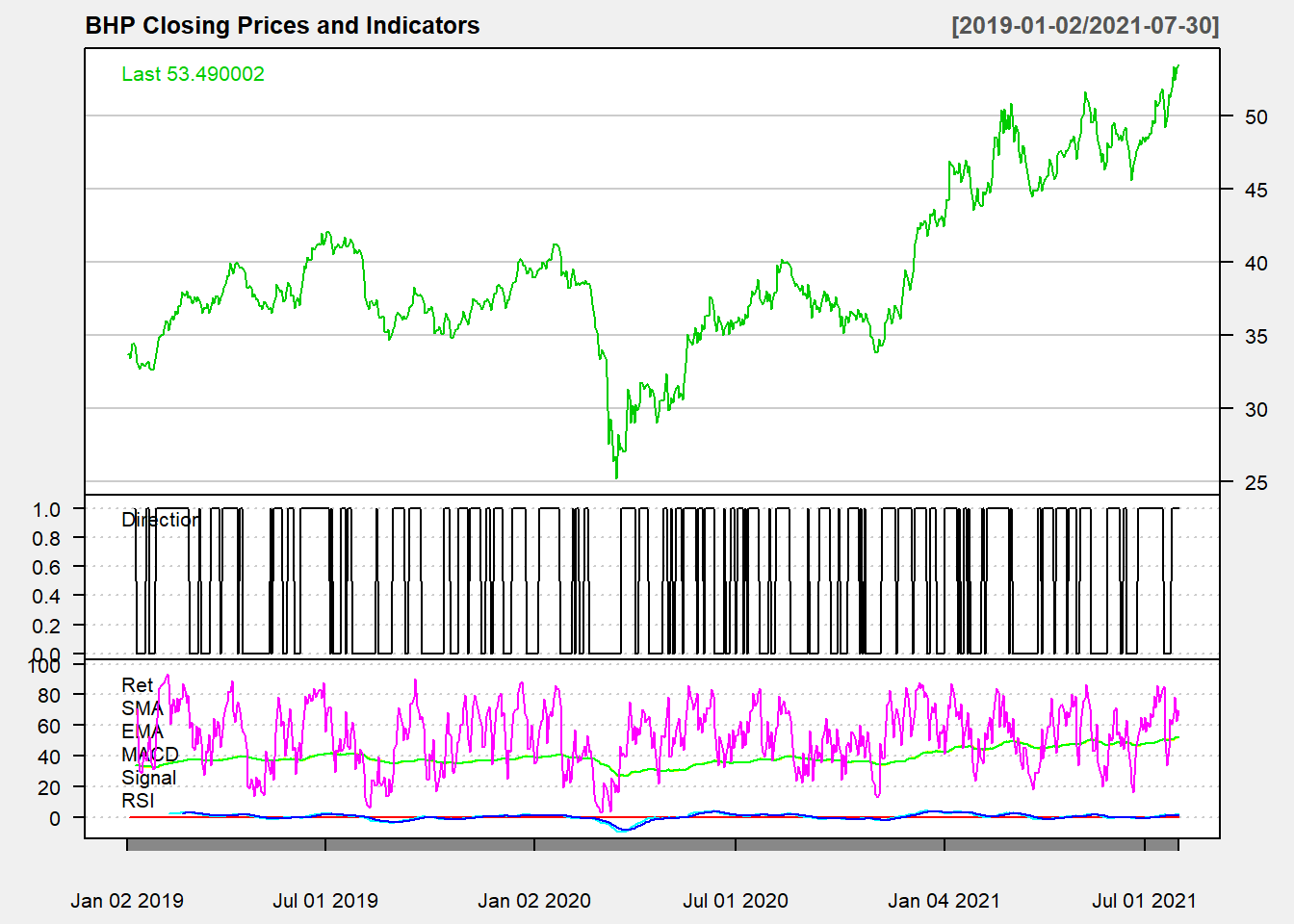

Figure 14.1: Direction and Technical Indicators

The above graph can be improved using ggplot2

library(tidyr)
library(ggplot2)
# create a dataset and convert data to long
d_plot = merge.xts(d_bhp, d_ex1)
# remove NAs and then convert to long

d_plot = na.omit(d_plot)
# convert to dataframe
d_plot = data.frame(Date = index(d_plot), coredata(d_plot))
d_plot_long = pivot_longer(d_plot, -c(Date, Direction), values_to = "value",
    names_to = "Indicator")

# change direction to a factor
d_plot_long$Direction = as.factor(d_plot_long$Direction)

(p2_ex = ggplot(d_plot_long, aes(Date, value, color = Indicator)) + geom_path(stat = "identity") +
    facet_grid(Indicator ~ ., scale = "free") + theme_minimal())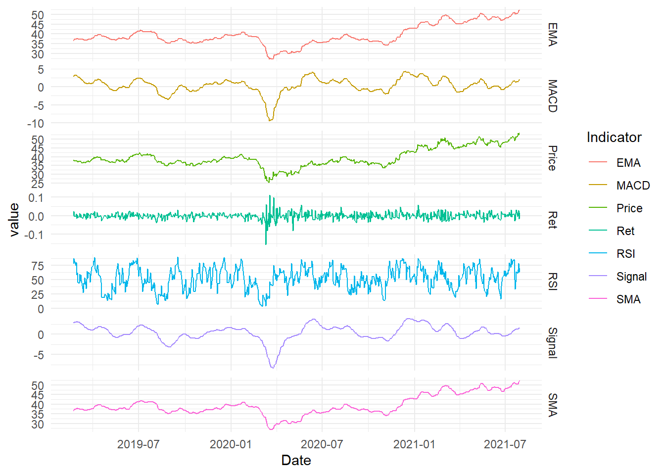

Figure 14.2: Indicators and Prices (ggplot2)

The above is a line chart of indicators and prices. We can also create a box plot to visualise the variance in the values relative to the direction

p2_ex = ggplot(d_plot_long, aes(value, Indicator, fill = Direction)) +
    geom_boxplot()

p2_ex + theme_minimal() + labs(title = "TA Indicators vs Price Direction") +
    scale_fill_manual(name = "Price Direction", values = c("orange", "lightblue"))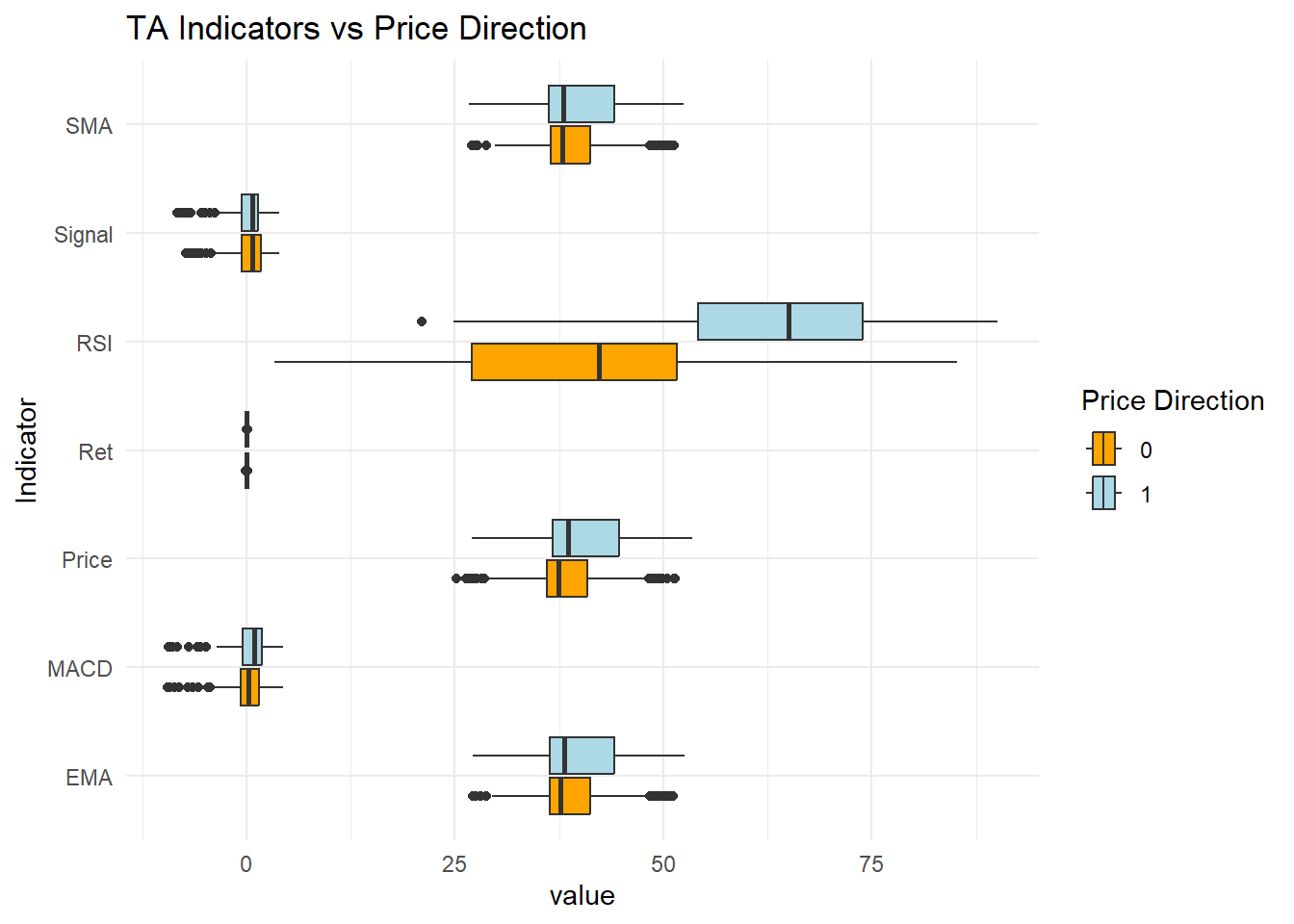

Figure 14.3: Box Plot of Indicators

Some differences per category can be noticed

14.3.3 Using Logistic Regression

70:30 data split
Time series sampling
- Stratified sampling will not keep the time order and hence its avoided

# remove NAs
d_ex1 = na.omit(d_ex1)
# convert to data frame
d_ex1 = as.data.frame(d_ex1)
# convert direction to a factor for classification

d_ex1$Direction = as.factor(d_ex1$Direction)

idx1 = c(1:round(nrow(d_ex1) * 0.7))  #create index for first 70% values to be in the testing set
d_train1 = d_ex1[idx1, ]  #training set
d_test1 = d_ex1[-idx1, ]  #testing set

Training Setup

Time series cross validate for resampling: 250 day window 30 days for prediction (this can be changed)
Data preprocessing is conducted to normalise the scale of the values
glm method with binomial family for the binary classification

library(caret)
set.seed(999)
# control
cntrl1 = trainControl(method = "timeslice", initialWindow = 250, horizon = 30,
    fixedWindow = TRUE)
# preprocesing
prep1 = c("center", "scale")
# logistic regression
logit_ex1 = train(Direction ~ ., data = d_train1, method = "glm", family = "binomial",
    trControl = cntrl1, preProcess = prep1)
logit_ex1  #final model accuracy

Generalized Linear Model 

434 samples
  6 predictor
  2 classes: '0', '1' 

Pre-processing: centered (6), scaled (6) 
Resampling: Rolling Forecasting Origin Resampling (30 held-out with a fixed window) 
Summary of sample sizes: 250, 250, 250, 250, 250, 250, ... 
Resampling results:

  Accuracy   Kappa    
  0.7324731  0.4658076

summary(logit_ex1$finalModel)  #summary of the final model


Call:
NULL

Deviance Residuals: 
     Min        1Q    Median        3Q       Max  
-2.43299  -0.63007  -0.04745   0.57603   2.49565  

Coefficients:
             Estimate Std. Error z value Pr(>|z|)    
(Intercept)  -0.05772    0.13429  -0.430    0.667    
Ret          -0.82494    0.18720  -4.407 1.05e-05 ***
SMA         -20.20397    3.70217  -5.457 4.83e-08 ***
EMA          20.05707    3.67374   5.460 4.77e-08 ***
MACD          0.50610    0.73203   0.691    0.489    
Signal       -0.94914    0.68541  -1.385    0.166    
RSI           2.14092    0.30037   7.128 1.02e-12 ***
---
Signif. codes:  0 '***' 0.001 '**' 0.01 '*' 0.05 '.' 0.1 ' ' 1

(Dispersion parameter for binomial family taken to be 1)

    Null deviance: 601.61  on 433  degrees of freedom
Residual deviance: 348.17  on 427  degrees of freedom
AIC: 362.17

Number of Fisher Scoring iterations: 5

Variable importance
In the case of multiple predictor variables, we want to understand which variable is the most influential in predicting the response variable.

library(vip)
vip(logit_ex1, geom = "point") + theme_minimal()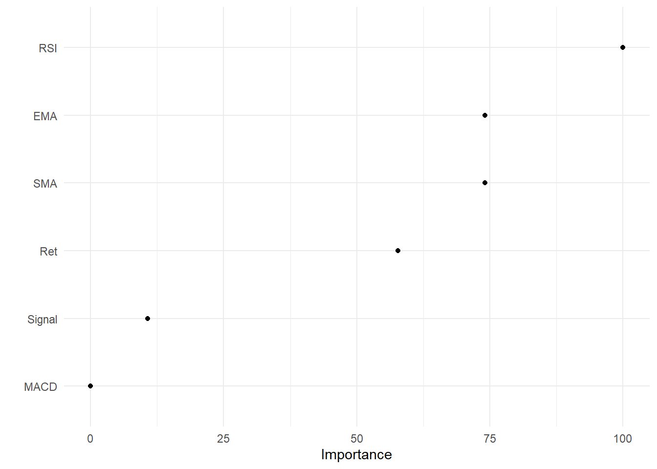

Figure 14.4: Variable Importance

Predictive Accuracy

ML models should be checked for predictive accuracy on the test set
caret provides predict function to create predictions
These predictions can be assessed based on the confusion matrix

Confusion Matrix - When applying classification models, we often use a confusion matrix to evaluate certain performance measures.

A confusion matrix is simply a matrix that compares actual categorical levels (or events) to the predicted categorical levels.
Prediction of the right level; refer to this as a true positive.
Prediction of a level or event that did not happen this is called a false positive (i.e. we predicted a customer would redeem a coupon and they did not).
Alternatively, when we do not predict a level or event and it does happen that this is called a false negative (i.e. a customer that we did not predict to redeem a coupon does).
Let’s predict using the final model and assess using the confusion matrix.

pred1 = predict(logit_ex1, newdata = d_test1)  #prediction on the test data
confusionMatrix(data = pred1, reference = d_test1$Direction)

Confusion Matrix and Statistics

          Reference
Prediction  0  1
         0 52 26
         1 16 92
                                          
               Accuracy : 0.7742          
                 95% CI : (0.7073, 0.8321)
    No Information Rate : 0.6344          
    P-Value [Acc > NIR] : 2.959e-05       
                                          
                  Kappa : 0.5279          
                                          
 Mcnemar's Test P-Value : 0.1649          
                                          
            Sensitivity : 0.7647          
            Specificity : 0.7797          
         Pos Pred Value : 0.6667          
         Neg Pred Value : 0.8519          
             Prevalence : 0.3656          
         Detection Rate : 0.2796          
   Detection Prevalence : 0.4194          
      Balanced Accuracy : 0.7722          
                                          
       'Positive' Class : 0

The model provides decent accuracy which is higher than the No Information Rate and also statistically significant.

There are other analyses which can be conducted on logistic regression, for example, ROC (Receiver Operating Characteristic) curve analysis for the Area Under the Curve.

14.3.4 Using K-NN

This section will implement the previous model using k-nearest neigbour algorithm using the caret package
Then we will use the same split as the logistic regression
We are selecting the model based on Accuracy & Kappa
Accuracy: Accuracy measures the overall correctness of the classifier \(\frac{(TN+TP)}{Total}\). Objective: maximise
Kappa (Cohen’s Kappa): Its like Accuracy but it is normalised at the baseline of random chance on the dataset. It compares observed accuracy to expected accuracy.
A grid search is used to search for an optimal value for k

set.seed(999)
grid1 = expand.grid(k = seq(1, 10, by = 2))  #to search from k=1 to k=10 
knn_ex1 = train(Direction ~ ., data = d_train1, method = "knn", tuneGrid = grid1,
    trControl = cntrl1, preProcess = prep1)

View the fit

plot(knn_ex1)  #may suggest using a wider grid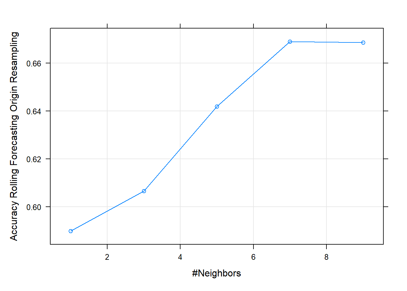

Figure 14.5: Grid plot

knn_ex1

k-Nearest Neighbors 

434 samples
  6 predictor
  2 classes: '0', '1' 

Pre-processing: centered (6), scaled (6) 
Resampling: Rolling Forecasting Origin Resampling (30 held-out with a fixed window) 
Summary of sample sizes: 250, 250, 250, 250, 250, 250, ... 
Resampling results across tuning parameters:

  k  Accuracy   Kappa    
  1  0.5898925  0.1554741
  3  0.6066667  0.1834679
  5  0.6419355  0.2500894
  7  0.6690323  0.3194890
  9  0.6686022  0.3209926

Accuracy was used to select the optimal model using the largest value.
The final value used for the model was k = 7.

Variable importance can’t be obtained here as KNN does not produce a model

Predictive Accuracy

Let’s predict using the final model and assess using the confusion matrix.

pred2 = predict(knn_ex1, newdata = d_test1)  #prediction on the test data
confusionMatrix(data = pred2, reference = d_test1$Direction)

Confusion Matrix and Statistics

          Reference
Prediction  0  1
         0 50 50
         1 18 68
                                          
               Accuracy : 0.6344          
                 95% CI : (0.5608, 0.7037)
    No Information Rate : 0.6344          
    P-Value [Acc > NIR] : 0.5330295       
                                          
                  Kappa : 0.2833          
                                          
 Mcnemar's Test P-Value : 0.0001704       
                                          
            Sensitivity : 0.7353          
            Specificity : 0.5763          
         Pos Pred Value : 0.5000          
         Neg Pred Value : 0.7907          
             Prevalence : 0.3656          
         Detection Rate : 0.2688          
   Detection Prevalence : 0.5376          
      Balanced Accuracy : 0.6558          
                                          
       'Positive' Class : 0

A comparison betweek Logistic Regression and KNN can be made based on their predictive accuracy.
The two models can also be compared based on their resampling results.
The random number seeds should be initialised to the same value for resampling comparison.
The following code compares the model fits.

resamp1 = resamples(list(logit = logit_ex1, knn = knn_ex1))

summary(resamp1)


Call:
summary.resamples(object = resamp1)

Models: logit, knn 
Number of resamples: 155 

Accuracy 
           Min.   1st Qu.    Median      Mean   3rd Qu.      Max. NA's
logit 0.4666667 0.6666667 0.7333333 0.7324731 0.8000000 0.9000000    0
knn   0.4333333 0.5666667 0.6666667 0.6690323 0.7666667 0.8666667    0

Kappa 
            Min.   1st Qu.    Median      Mean   3rd Qu.      Max. NA's
logit  0.1208791 0.3333333 0.4666667 0.4658076 0.5838144 0.7887324    0
knn   -0.1860465 0.1558442 0.3243243 0.3194890 0.4666667 0.7235023    0

bwplot(resamp1, metric = "Accuracy")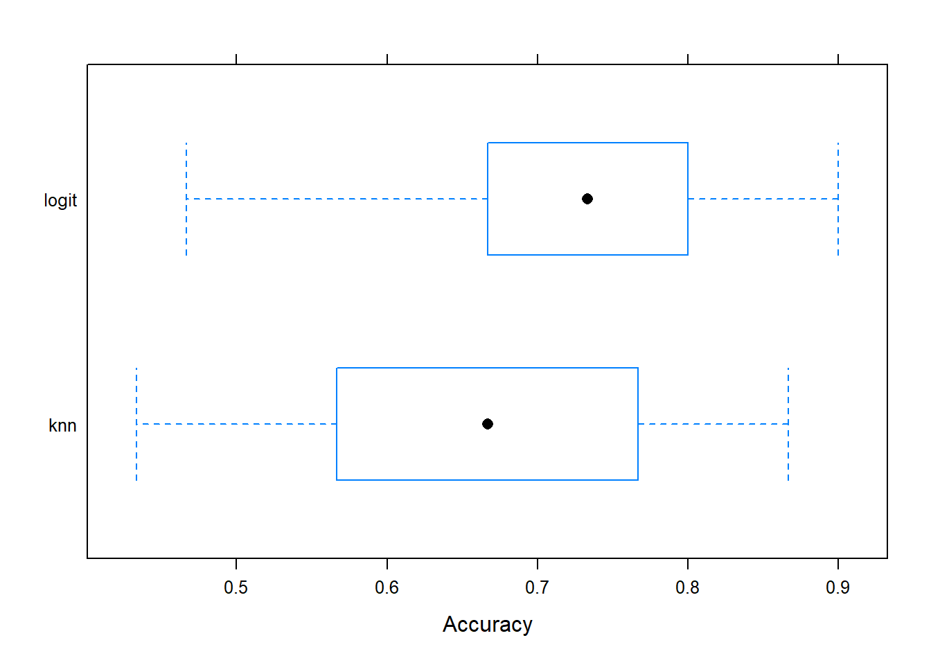

Figure 14.6: Resample Accuracy comparison

The graph provides a comparison of the overall accuracy of the model (not the predictions).

References

Boehmke, B., & Greenwell, B. M. (2019). Hands-on machine learning with r. CRC Press. Retrieved from https://bradleyboehmke.github.io/HOML/

Hastie, T., Tibshirani, R., James, G., & Witten, D. (2013). An introduction to statistical learning with applications in r. Springer New York.

Shynkevich, Y., McGinnity, T. M., Coleman, S. A., Belatreche, A., & Li, Y. (2017). Forecasting price movements using technical indicators: Investigating the impact of varying input window length. Neurocomputing, 264, 71–88. https://doi.org/https://doi.org/10.1016/j.neucom.2016.11.095