Topic 15 Decision Trees using R

Some references: Boehmke & Greenwell (2019), Hastie et al. (2013) and Lantz (2019)
In this section we discuss tree based methods for classification.
Tree-based models are a class of non-parametric algorithms that work by partitioning the feature space into a number of smaller (non-overlapping) regions with similar response values using a set of splitting rules.
These involve stratifying or segmenting the predictor space into a number of simple regions.
Typically use the mean or the mode of the training observations in the region to which it belongs.
Since the set of splitting rules used to segment the predictor space can be summarized in a tree, these types of approaches are known as decision tree methods.
Classification and Regression Tree (CART) (Breiman, Friedman, Stone, & Olshen (1984)) is the most well-known decision tree algorithm.
- CART uses binary recursive partitioning: Each split depends on the split above (before) it.
A basic decision tree partitions the training data into homogeneous subgroups (i.e., groups with similar response values) and then fits a simple constant in each subgroup (e.g., the mean of the within group response values for regression).
The subgroups (also called nodes) are formed recursively using binary partitions formed by asking simple yes-or-no questions about each feature.
This is done a number of times until a suitable stopping criteria is satisfied (e.g., a maximum depth of the tree is reached).
After all the partitioning has been done, the model predicts the output based on
- the average response values for all observations that fall in that subgroup (regression problem), or
- the class that has majority representation (classification problem)
Root node: First subgroup
Terminal node or Leaf node: Final subgroup
Internal node: Other subgroups between root and terminal node
Branches: Connection between the nodes
We will apply the CART method on a Credit Risk Example
Two types of risks are associated with the bank’s decision
- If the applicant is a good credit risk, i.e. is likely to repay the loan, then not approving the loan to the person results in a loss of business to the bank
- If the applicant is a bad credit risk, i.e. is not likely to repay the loan, then approving the loan to the person results in a financial loss to the bank
This analysis is an example and is not exhaustive list of methods available for data description, visualisation or ML using R.
15.1 Import Data and Pre-processing
Data discription is here https://onlinecourses.science.psu.edu/stat508/book/export/html/796
20 variables
Status of existing checking account. Duration in month Credit history Purpose Credit amount Savings account/bonds Present employment since Installment rate in percentage of disposable income Personal status and sex Other debtors / guarantors Present residence since Property Age in years Other installment plans Housing Number of existing credits at this bank Job Number of people being liable to provide maintenance for Telephone foreign worker
data_cr = read.csv("data/german_credit.csv")
# preliminary analysis descriptive and visual
str(data_cr)
'data.frame': 1000 obs. of 21 variables:
$ Creditability : int 1 1 1 1 1 1 1 1 1 1 ...
$ Account.Balance : int 1 1 2 1 1 1 1 1 4 2 ...
$ Duration.of.Credit..month. : int 18 9 12 12 12 10 8 6 18 24 ...
$ Payment.Status.of.Previous.Credit: int 4 4 2 4 4 4 4 4 4 2 ...
$ Purpose : int 2 0 9 0 0 0 0 0 3 3 ...
$ Credit.Amount : int 1049 2799 841 2122 2171 2241 3398 1361 1098 3758 ...
$ Value.Savings.Stocks : int 1 1 2 1 1 1 1 1 1 3 ...
$ Length.of.current.employment : int 2 3 4 3 3 2 4 2 1 1 ...
$ Instalment.per.cent : int 4 2 2 3 4 1 1 2 4 1 ...
$ Sex...Marital.Status : int 2 3 2 3 3 3 3 3 2 2 ...
$ Guarantors : int 1 1 1 1 1 1 1 1 1 1 ...
$ Duration.in.Current.address : int 4 2 4 2 4 3 4 4 4 4 ...
$ Most.valuable.available.asset : int 2 1 1 1 2 1 1 1 3 4 ...
$ Age..years. : int 21 36 23 39 38 48 39 40 65 23 ...
$ Concurrent.Credits : int 3 3 3 3 1 3 3 3 3 3 ...
$ Type.of.apartment : int 1 1 1 1 2 1 2 2 2 1 ...
$ No.of.Credits.at.this.Bank : int 1 2 1 2 2 2 2 1 2 1 ...
$ Occupation : int 3 3 2 2 2 2 2 2 1 1 ...
$ No.of.dependents : int 1 2 1 2 1 2 1 2 1 1 ...
$ Telephone : int 1 1 1 1 1 1 1 1 1 1 ...
$ Foreign.Worker : int 1 1 1 2 2 2 2 2 1 1 ...# remove NA
data_cr = na.omit(data_cr)
# quick summary
summary(data_cr) Creditability Account.Balance Duration.of.Credit..month.
Min. :0.0 Min. :1.000 Min. : 4.0
1st Qu.:0.0 1st Qu.:1.000 1st Qu.:12.0
Median :1.0 Median :2.000 Median :18.0
Mean :0.7 Mean :2.577 Mean :20.9
3rd Qu.:1.0 3rd Qu.:4.000 3rd Qu.:24.0
Max. :1.0 Max. :4.000 Max. :72.0
Payment.Status.of.Previous.Credit Purpose Credit.Amount
Min. :0.000 Min. : 0.000 Min. : 250
1st Qu.:2.000 1st Qu.: 1.000 1st Qu.: 1366
Median :2.000 Median : 2.000 Median : 2320
Mean :2.545 Mean : 2.828 Mean : 3271
3rd Qu.:4.000 3rd Qu.: 3.000 3rd Qu.: 3972
Max. :4.000 Max. :10.000 Max. :18424
Value.Savings.Stocks Length.of.current.employment Instalment.per.cent
Min. :1.000 Min. :1.000 Min. :1.000
1st Qu.:1.000 1st Qu.:3.000 1st Qu.:2.000
Median :1.000 Median :3.000 Median :3.000
Mean :2.105 Mean :3.384 Mean :2.973
3rd Qu.:3.000 3rd Qu.:5.000 3rd Qu.:4.000
Max. :5.000 Max. :5.000 Max. :4.000
Sex...Marital.Status Guarantors Duration.in.Current.address
Min. :1.000 Min. :1.000 Min. :1.000
1st Qu.:2.000 1st Qu.:1.000 1st Qu.:2.000
Median :3.000 Median :1.000 Median :3.000
Mean :2.682 Mean :1.145 Mean :2.845
3rd Qu.:3.000 3rd Qu.:1.000 3rd Qu.:4.000
Max. :4.000 Max. :3.000 Max. :4.000
Most.valuable.available.asset Age..years. Concurrent.Credits
Min. :1.000 Min. :19.00 Min. :1.000
1st Qu.:1.000 1st Qu.:27.00 1st Qu.:3.000
Median :2.000 Median :33.00 Median :3.000
Mean :2.358 Mean :35.54 Mean :2.675
3rd Qu.:3.000 3rd Qu.:42.00 3rd Qu.:3.000
Max. :4.000 Max. :75.00 Max. :3.000
Type.of.apartment No.of.Credits.at.this.Bank Occupation No.of.dependents
Min. :1.000 Min. :1.000 Min. :1.000 Min. :1.000
1st Qu.:2.000 1st Qu.:1.000 1st Qu.:3.000 1st Qu.:1.000
Median :2.000 Median :1.000 Median :3.000 Median :1.000
Mean :1.928 Mean :1.407 Mean :2.904 Mean :1.155
3rd Qu.:2.000 3rd Qu.:2.000 3rd Qu.:3.000 3rd Qu.:1.000
Max. :3.000 Max. :4.000 Max. :4.000 Max. :2.000
Telephone Foreign.Worker
Min. :1.000 Min. :1.000
1st Qu.:1.000 1st Qu.:1.000
Median :1.000 Median :1.000
Mean :1.404 Mean :1.037
3rd Qu.:2.000 3rd Qu.:1.000
Max. :2.000 Max. :2.000 - Let’s convert data types to as all of them are factors but some of them should be used as numeric
sapply(data_cr, class) Creditability Account.Balance
"integer" "integer"
Duration.of.Credit..month. Payment.Status.of.Previous.Credit
"integer" "integer"
Purpose Credit.Amount
"integer" "integer"
Value.Savings.Stocks Length.of.current.employment
"integer" "integer"
Instalment.per.cent Sex...Marital.Status
"integer" "integer"
Guarantors Duration.in.Current.address
"integer" "integer"
Most.valuable.available.asset Age..years.
"integer" "integer"
Concurrent.Credits Type.of.apartment
"integer" "integer"
No.of.Credits.at.this.Bank Occupation
"integer" "integer"
No.of.dependents Telephone
"integer" "integer"
Foreign.Worker
"integer" # Keep Duration.of.Credit..month and Credit.Amount as numeric rest to
# factors
id = c(1, 2, 4, 5, 7:21)
data_cr[id] = lapply(data_cr[id], as.factor)15.2 Visualisation some features
Create some visualisation to visualise data characteristics
Box plots 15.1 for Duration of Credit and Credit Amount
library(ggplot2)
library(gridExtra)
# copy of data for plots
data_cr_p = data_cr
# set theme for the session
theme_set(theme_bw())
p1 = ggplot(data_cr, aes(Duration.of.Credit..month., fill = Creditability)) +
    geom_boxplot()
p2 = ggplot(data_cr_p, aes(Credit.Amount, Creditability, fill = Creditability)) +
    geom_boxplot()

grid.arrange(p1, p2, ncol = 1)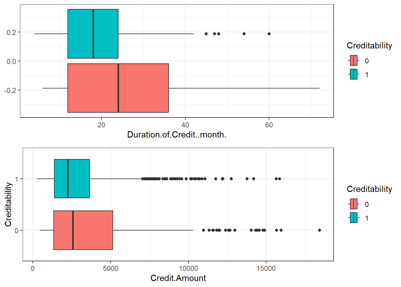
Figure 15.1: Box Plots
- See the relationship between Purpose, Sex/status and Creditability 15.2
p3 = ggplot(data_cr_p, aes(Purpose)) + geom_bar(aes(fill = Creditability),
    stat = "count", position = "dodge")

p4 = ggplot(data_cr_p, aes(Sex...Marital.Status)) + geom_bar(aes(fill = Creditability),
    stat = "count", position = "dodge")

grid.arrange(p3, p4, ncol = 2)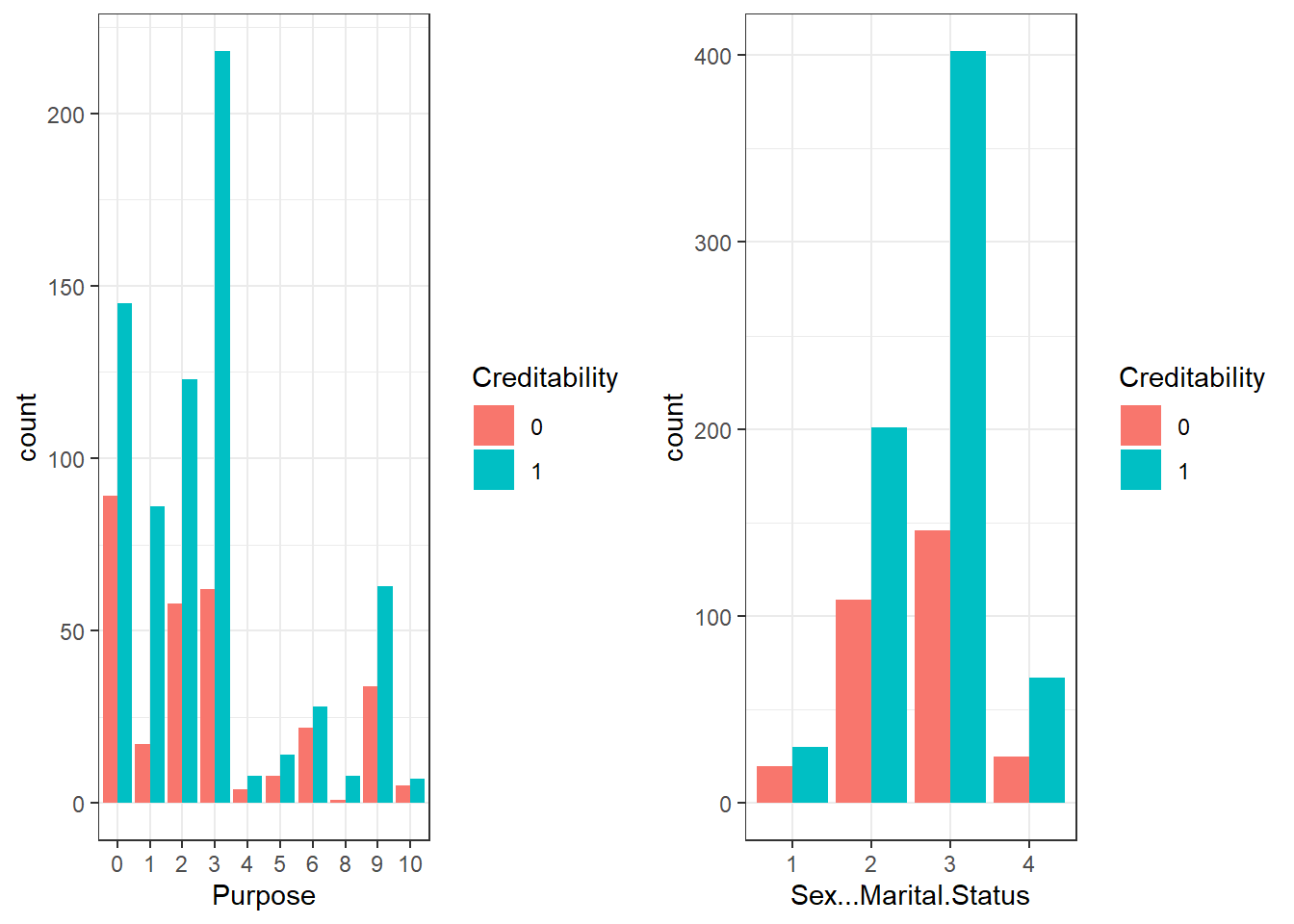
Figure 15.2: Bar plots
15.3 Creating Training and Testing Set and Control
- Use rsample package and stratified sampling
- Using mutliple cross validation for resampling
library(rsample)
library(caret)
set.seed(999)  #for reproducibility (can pick your own seed, but keep it consistent)
idx = initial_split(data = data_cr, prop = 0.8, strata = "Creditability")
d_train1 = training(idx)
d_test1 = testing(idx)
prop.table(table(d_train1$Creditability))
  0   1
0.3 0.7 prop.table(table(d_test1$Creditability))
  0   1
0.3 0.7
cntrl1 = trainControl(method = "repeatedcv", number = 10, repeats = 2) #using repeated cross validate (repeating twice)15.4 Train the model on the training set
Use rpart package and caret package
The following block may results in slightly different results on individual computers. The fitted models are in data folder
set.seed(999)  #for reproducibility
cv_tree1 = train(Creditability ~ ., data = d_train1, trControl = cntrl1,
    method = "rpart", tuneLength = 20, parms = list(split = "gini"))  #using gini index
cv_tree2 = train(Creditability ~ ., data = d_train1, trControl = cntrl1,
    method = "rpart", tuneLength = 20, parms = list(split = "information"))  #using information
The fitted models were saved afterwards as cv_tree1_gini.Rdata and cv_tree2_info.Rdata
Loading the fitted models to analyse
set.seed(999)
load("data/cv_tree1_gini.Rdata")
load("data/cv_tree2_info.Rdata")
# model fit 1
cv_tree1
CART
802 samples
20 predictor
2 classes: '0', '1'
No pre-processing
Resampling: Cross-Validated (10 fold, repeated 2 times)
Summary of sample sizes: 721, 722, 722, 722, 722, 721, ...
Resampling results across tuning parameters:
cp Accuracy Kappa
0.000000000 0.6969830 0.2512465
0.001747106 0.6988580 0.2543412
0.003494213 0.7063349 0.2628946
0.005241319 0.7206867 0.2861502
0.006988425 0.7200540 0.2777666
0.008735532 0.7200617 0.2727974
0.010482638 0.7244367 0.2758523
0.012229744 0.7219444 0.2739317
0.013976851 0.7256636 0.2964605
0.015723957 0.7262886 0.2940382
0.017471064 0.7262886 0.2936297
0.019218170 0.7238272 0.2881274
0.020965276 0.7225926 0.2839374
0.022712383 0.7225926 0.2839374
0.024459489 0.7151466 0.2534916
0.026206595 0.7145370 0.2595461
0.027953702 0.7070833 0.2284884
0.029700808 0.7014583 0.2203101
0.031447914 0.6983565 0.1916670
0.033195021 0.6902701 0.1609005
Accuracy was used to select the optimal model using the largest value.
The final value used for the model was cp = 0.01747106.# model fit 2
cv_tree2CART
802 samples
20 predictor
2 classes: '0', '1'
No pre-processing
Resampling: Cross-Validated (10 fold, repeated 2 times)
Summary of sample sizes: 721, 722, 722, 722, 721, 722, ...
Resampling results across tuning parameters:
cp Accuracy Kappa
0.000000000 0.6963735 0.2470114
0.001747106 0.7056867 0.2628565
0.003494213 0.7050849 0.2532738
0.005241319 0.7056867 0.2530103
0.006988425 0.7144290 0.2708436
0.008735532 0.7144290 0.2715985
0.010482638 0.7200540 0.2804530
0.012229744 0.7237654 0.2784178
0.013976851 0.7275154 0.2885322
0.015723957 0.7231404 0.2833342
0.017471064 0.7237731 0.2843818
0.019218170 0.7243981 0.2782958
0.020965276 0.7237886 0.2732868
0.022712383 0.7237886 0.2732868
0.024459489 0.7225386 0.2708625
0.026206595 0.7144136 0.2456549
0.027953702 0.7082022 0.2211492
0.029700808 0.7082022 0.2211492
0.031447914 0.7013580 0.1774435
0.033195021 0.6976080 0.1496378
Accuracy was used to select the optimal model using the largest value.
The final value used for the model was cp = 0.01397685.plot(cv_tree1) #parameter search using gini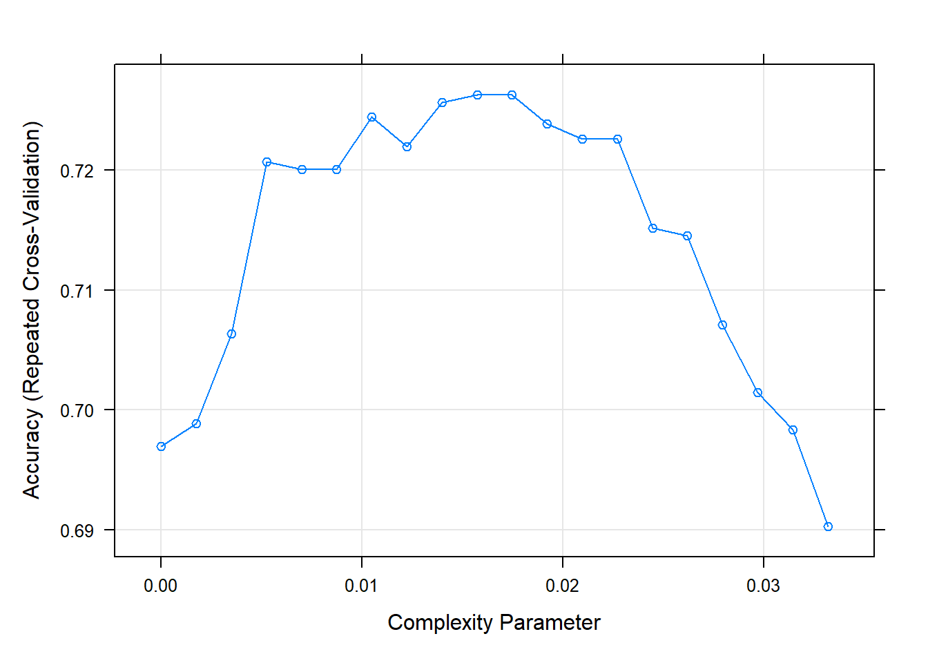
plot(cv_tree2) #parameter search using information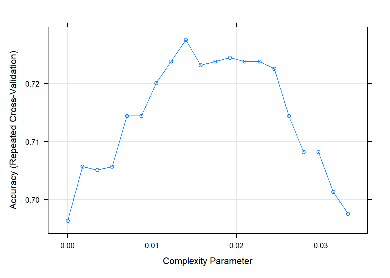
15.5 Prediction and Accuracy
- Using testing set and confusion matrix to compare accuracies
15.5.1 Model-1
pred1 = predict(cv_tree1, newdata = d_test1)
confusionMatrix(pred1, d_test1$Creditability)
Confusion Matrix and Statistics
Reference
Prediction 0 1
0 33 10
1 27 130
Accuracy : 0.815
95% CI : (0.7541, 0.8663)
No Information Rate : 0.7
P-Value [Acc > NIR] : 0.0001479
Kappa : 0.5207
Mcnemar's Test P-Value : 0.0085289
Sensitivity : 0.5500
Specificity : 0.9286
Pos Pred Value : 0.7674
Neg Pred Value : 0.8280
Prevalence : 0.3000
Detection Rate : 0.1650
Detection Prevalence : 0.2150
Balanced Accuracy : 0.7393
'Positive' Class : 0
15.5.2 Model-2
pred2 = predict(cv_tree2, newdata = d_test1)
confusionMatrix(pred2, d_test1$Creditability)
Confusion Matrix and Statistics
Reference
Prediction 0 1
0 32 9
1 28 131
Accuracy : 0.815
95% CI : (0.7541, 0.8663)
No Information Rate : 0.7
P-Value [Acc > NIR] : 0.0001479
Kappa : 0.5157
Mcnemar's Test P-Value : 0.0030846
Sensitivity : 0.5333
Specificity : 0.9357
Pos Pred Value : 0.7805
Neg Pred Value : 0.8239
Prevalence : 0.3000
Detection Rate : 0.1600
Detection Prevalence : 0.2050
Balanced Accuracy : 0.7345
'Positive' Class : 0