Topic 2 R Data Types and Data Structures
When human judgement and big data intersect there are some funny things that happen. -Nate Silver
2.1 Data Types
As per R’s official language definitions; in every computer language variables provide a means of accessing the data stored in memory.
R does not provide direct access to the computer’s memory but rather provides a number of specialized data structures we will refer to as objects. These objects are referred to through symbols or variables.
2.1.1 Double
- Doubles are numbers like 5.0, 5.5, 10.999 etc. They may or may not include decimal places. Doubles are mostly used to represent a continuous variable like serial number, weight, age etc.
x = 8.5
is.double(x)  #to check if the data type is double
[1] TRUE2.1.2 Integer
- Integers are natural numbers.
x = 9
typeof(x)
[1] "double"# The following specifically assigns an integer to x
x = as.integer(9)
typeof(x)[1] "integer"2.1.3 Logical
- A variable of data type logical has the value TRUE or FALSE. To perform calculation on logical objects in R the FALSE is replaced by a zero and TRUE is replaced by 1.
x = 11
y = 10
a = x > y
a
[1] TRUEtypeof(a)[1] "logical"2.1.4 Character
- Characters represent the string values in R. An object of type character can have alphanumeric strings. Character objects are specified by assigning a string or collection of characters between double quotes (“ string”) . Everything in a double quote is considered a string in R.
2.1.5 Factor
-Factor is an important data type to represent categorical data. This also comes handy when dealing with Panel or Longitudinal data. Example of factors are Blood type (A , B, AB, O), Sex (Male or Female). Factor objects can be created from character object or from numeric object. -The operator c is used to create a vector of values which can be of any data type.
b.type = c("A", "AB", "B", "O")  #character object
# use factor function to convert to factor object
b.type = factor(b.type)
b.type
[1] A AB B O
Levels: A AB B O# to get individual elements (levels) in factor object
levels(b.type)[1] "A" "AB" "B" "O" 2.1.6 Date & Time
-R is capable of dealing calendar dates and times. It is an important object when dealing with time series models. The function as.Date can be used to create an object of class Date.
- see help(as.Date) for more details about the format of dates.
date1 = "31-01-2012"
date1 = as.Date(date1, "%d-%m-%Y")
date1
[1] "2012-01-31"data.class(date1)[1] "Date"# The date and time are internally interpreted as Double so the function typeof
# will return the type Double
typeof(date1)[1] "double"2.2 Data Structures in R
Every data analysis requires the data to be structured in a well defined way. These coherent ways to put together data forms some basic data structures in R. Every data set intended for analysis has to be imported in R environment as a data structure. R has the following basic data structures:
• Vector
• Matrix
• Array
• Data Frame
• Lists
2.2.1 Vector
Vectors are group of values having same data types.
There can be numeric vectors, character vector and so on. Vectors are mostly used to represent a single variable in a data set.
A vector is constructed using the function
c. The same functionccan be used to combine different vectors of same data type.
vec1 = c(1, 2, 3, 4, 5)
vec1
[1] 1 2 3 4 5The
strfunction can be used to view the data structure of an object
2.2.2 Matrices
- A matrix is a collection of data elements arranged in a two-dimensional rectangular layout. Like vectors all the elements in a matrix are of same data type.
\[\left[\begin{array}{cc} 1 & 2\\ 3 & 4\\ 5 & 6 \end{array}\right]\]
- The function \(\mathtt{matrix}\) is used to create matrices in R. Note that all the elements in a matrix object are of same basic type. Lets create the matrix in the example above.
m1 = matrix(c(1, 2, 3, 4, 5, 6), nrow = 3, ncol = 2, byrow = TRUE)
# nrow-specify number of rows, ncol-specify number of columns, byrow-fill the
# matrix in rows with the data supplied
m1  #print the matrix
[,1] [,2]
[1,] 1 2
[2,] 3 4
[3,] 5 6- A vector can be converted to matrix using \(\mathtt{dim}\) function, e.g:
m2 = c(1, 2, 3, 4, 5, 6)
dim(m2) = c(3, 2)  #the matrix will be filled by columns
m2
[,1] [,2]
[1,] 1 4
[2,] 2 5
[3,] 3 6# use dim to get the dimension (#rows and #columns) of a matrix
dim(m1)[1] 3 2** Matrix Manipulations **
- For calculations on matrices; all the mathematical functions available for vectors are applicable on a matrix. All operations are applied on each element in a matrix, e.g.
m3 = m1 * 2  # all elements will be multiplied by 2 individually
m3
[,1] [,2]
[1,] 2 4
[2,] 6 8
[3,] 10 12A matrix can be multiplied with a vector as long as the length of the vector is a multiple of length of the matrix. Try different combinations of matrix and vector arithmetic to see the results and errors.
Mathematical matrix operations are also available for matrices in R. For instance \(\mathtt{\%*\%}\) is used for matrix multiplication, the matrices must agree dimensionally for matrix multiplication. Note the use of \(\mathtt{:}\) operator to create a sequence.
dim(m1) # 3 rows and 2 columns[1] 3 2# create another matrix with 2 rows and 3 columns
m3 = matrix(c(1:6), ncol = 3)
m1 %*% m3 [,1] [,2] [,3]
[1,] 5 11 17
[2,] 11 25 39
[3,] 17 39 61R facilitates various matrix specific operations. Table 1 gives most of the available functions and operators. Use \(\mathtt{help()}\) or \(\mathtt{?}\) followed by function name to get more details about the operators and functions.
|
Operator or Function
|
Description
|
|
X * Y
|
Element-wise multiplication
|
|
X %*% Y
|
Matrix multiplication
|
|
Y %o% X
|
Outer product. XB’
|
|
crossprod(X,Y)
|
X’Y
|
|
crossprod(X)
|
X’X
|
|
t(X)
|
Transpose
|
|
diag(x)
|
Creates diagonal matrix with elements of x in the principal diagonal
|
|
diag(X)
|
Returns a vector containing the elements of the principal diagonal
|
|
diag(k)
|
If k is a scalar, this creates a k x k identity matrix. Go figure.
|
|
solve(X, b)
|
Returns vector x in the equation b = Xx (i.e., X-1b)
|
|
solve(X)
|
Inverse of X where X is a square matrix.
|
|
y=eigen(X)
|
y$val are the eigenvalues of X
|
|
y$vec are the eigenvectors of X
|
|
|
y=svd(X)
|
Singular value decomposition of X.
|
|
R = chol(X)
|
Choleski factorization of X. Returns the upper triangular factor, such that R’R = X.
|
|
y = qr(X)
|
QR decomposition of X.
|
|
cbind(X,Y,…)
|
Combine matrices(vectors) horizontally. Returns a matrix.
|
|
rbind(X,Y,…)
|
Combine matrices(vectors) vertically. Returns a matrix.
|
|
rowMeans(X)
|
Returns vector of row means.
|
|
rowSums(X)
|
Returns vector of row sums.
|
|
colMeans(X)
|
Returns vector of column means.
|
|
colSums(X)
|
Returns vector of column means.
|
2.2.3 Arrays
- Arrays are the generalisation of vectors and matrices. A vector in R is a one dimensional array and a matrix a two dimensional array. An array is a multiply subscripted collection of data entries of the same data type. Arrays can be constructed using the function \(\mathtt{array}\), for example5
z = c(1:24)  #vector of length 24
# constructing a 3 by 4 by 2 array
a1 = array(z, dim = c(3, 4, 2))
a1
, , 1
[,1] [,2] [,3] [,4]
[1,] 1 4 7 10
[2,] 2 5 8 11
[3,] 3 6 9 12
, , 2
[,1] [,2] [,3] [,4]
[1,] 13 16 19 22
[2,] 14 17 20 23
[3,] 15 18 21 24- Individual elements of an array are accessed by referring them by their index. This is done by giving the name of the array followed by the subscript (index) in this square bracket separated by commas. We try to access the element [1,3,1] of array a1 in the following example
# element in the row 1 and column 3 in the first subset
a1[1, 3, 1]
[1] 72.2.4 Data Frames
Data frame forms the most convenient data structures in R to represent tabular data.
In quantitative research data is often in the form of data tables. These data tables have multiple rows and can have multiple columns with each column representing a different variable (quantity).
A data frame in R is the most natural way to represent these data sets as it can have different data type in the data frame object. Most statistical routines in R require a data frame as input.
The following example uses an important function \(\mathtt{str}\) on R’s inbuilt data frame “swiss”. \(\mathtt{str}\) function is used to see the internal structure of an object in R.
options(str = list(vec.len = 2))
# swiss dataframe has standardized fertility measure and socio-economic
# indicators for each of 47 French-speaking provinces of Switzerland at about
# 1888.
data(swiss)
str(swiss)
'data.frame': 47 obs. of 6 variables:
$ Fertility : num 80.2 83.1 92.5 85.8 76.9 ...
$ Agriculture : num 17 45.1 39.7 36.5 43.5 ...
$ Examination : int 15 6 5 12 17 ...
$ Education : int 12 9 5 7 15 ...
$ Catholic : num 9.96 84.84 ...
$ Infant.Mortality: num 22.2 22.2 20.2 20.3 20.6 ...- Data frames have two attributes namely; \(\mathtt{names}\) and \(\mathtt{row.names}\), these two contains the column names and row names respectively. The data in the named column can be accessed by the \(\mathtt{\$}\) operator.
# using names and row.names
names(swiss)  #name of the columns (can also use colnames)
[1] "Fertility" "Agriculture" "Examination" "Education"
[5] "Catholic" "Infant.Mortality"colnames(swiss)[1] "Fertility" "Agriculture" "Examination" "Education"
[5] "Catholic" "Infant.Mortality"row.names(swiss) #name of the rows [1] "Courtelary" "Delemont" "Franches-Mnt" "Moutier" "Neuveville"
[6] "Porrentruy" "Broye" "Glane" "Gruyere" "Sarine"
[11] "Veveyse" "Aigle" "Aubonne" "Avenches" "Cossonay"
[16] "Echallens" "Grandson" "Lausanne" "La Vallee" "Lavaux"
[21] "Morges" "Moudon" "Nyone" "Orbe" "Oron"
[26] "Payerne" "Paysd'enhaut" "Rolle" "Vevey" "Yverdon"
[31] "Conthey" "Entremont" "Herens" "Martigwy" "Monthey"
[36] "St Maurice" "Sierre" "Sion" "Boudry" "La Chauxdfnd"
[41] "Le Locle" "Neuchatel" "Val de Ruz" "ValdeTravers" "V. De Geneve"
[46] "Rive Droite" "Rive Gauche" swiss$Fertility #returns the vector of data in the column Fertility [1] 80.2 83.1 92.5 85.8 76.9 76.1 83.8 92.4 82.4 82.9 87.1 64.1 66.9 68.9 61.7
[16] 68.3 71.7 55.7 54.3 65.1 65.5 65.0 56.6 57.4 72.5 74.2 72.0 60.5 58.3 65.4
[31] 75.5 69.3 77.3 70.5 79.4 65.0 92.2 79.3 70.4 65.7 72.7 64.4 77.6 67.6 35.0
[46] 44.7 42.8- Data frames are constructed using the function \(\mathtt{data.frame}\). For example following creates a data frame of a character and numeric vector.
num1 = seq(1:5)
ch1 = c("A", "B", "C", "D", "E")
df1 = data.frame(ch1, num1)
df1
ch1 num1
1 A 1
2 B 2
3 C 3
4 D 4
5 E 52.2.5 Lists
A list is like generic vector containing other objects. Lists can have numerous elements any type and structure they can also be of different lengths
A list can contain another list and therefore it can be used to construct arbitrary data structures.
A list can be constructed using the \(\mathtt{list}\) function, for example
e1 = c(2, 3, 5)  #element-1
e2 = c("aa", "bb", "cc", "dd", "ee")  #element-2
e3 = c(TRUE, FALSE, TRUE, FALSE, FALSE)  #element-3
e4 = df1  #element-4 (previously constructed data frame)
lst1 = list(e1, e2, e3, e4)  # lst contains copies of e1,e2,e3,e4
str(lst1)  #show the structure of lst1
List of 4
$ : num [1:3] 2 3 5
$ : chr [1:5] "aa" "bb" ...
$ : logi [1:5] TRUE FALSE TRUE ...
$ :'data.frame': 5 obs. of 2 variables:
..$ ch1 : chr [1:5] "A" "B" ...
..$ num1: int [1:5] 1 2 3 4 5- Components are always numbered and may always be referred to as such.
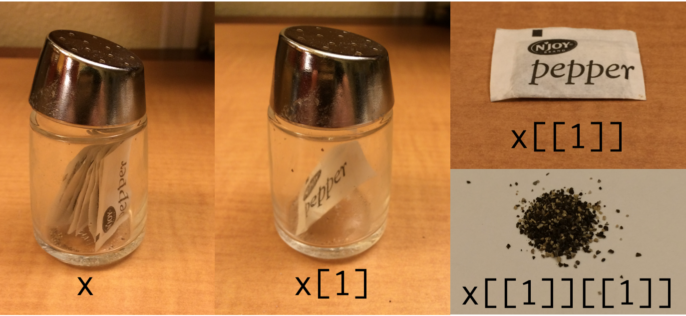
Figure 2.1: Lists
- Thus if lst1 is the name of a list with four components, these may be individually referred to as lst1[[1]], lst1[[2]], lst1[[3]] and lst1[[4]]. Note: When a single square bracket is used the component of a list is returned as a list while the double square bracket returns the component itself
# first element of lst1
lst1[[1]]
[1] 2 3 5lst1[1][[1]]
[1] 2 3 5- The elements in a list can also be named using the function and these elements can be referred individually via there names.
names(lst1) = c("e1", "e2", "e3", "e4")
names(lst1)  #name of the elements
[1] "e1" "e2" "e3" "e4"lst1$e1 #using $operator to refer the element[1] 2 3 5This section provided an overview of various data types and data structures in R. The next section will discuss how to deal with external data souces with flat data.
2.3 Data Import/Export in R
2.3.1 Reading Data from a Text File
The easiest way to import data into R’s statistical system is to do in a tabular format saved in a text/ file.
To import tabular data from a text file, R provides the function \(\mathtt{read.table()}\). \(\mathtt{read.table()}\) is the most convenient function to import tabular data from text files and can be easily used for data files of small or moderate size having data in a rectangular format. The arguments which can be passed to \(\mathtt{read.table()}\) are given below.
args(read.table)function (file, header = FALSE, sep = "", quote = "\"'", dec = ".",
numerals = c("allow.loss", "warn.loss", "no.loss"), row.names,
col.names, as.is = !stringsAsFactors, na.strings = "NA",
colClasses = NA, nrows = -1, skip = 0, check.names = TRUE,
fill = !blank.lines.skip, strip.white = FALSE, blank.lines.skip = TRUE,
comment.char = "#", allowEscapes = FALSE, flush = FALSE,
stringsAsFactors = FALSE, fileEncoding = "", encoding = "unknown",
text, skipNul = FALSE)
NULL- Some of the important arguments for the function \(\mathtt{read.table}\) are discussed below, for the rest see the help file using \(\mathtt{help(read.table)}\).
|
Argument
|
Description
|
|
file
|
The name of the tabular (text) file to import along with the full path
|
|
header
|
A logical argument to specify if the names of the variables are available in the first row
|
|
sep
|
Character to specify the seperator type, default “ “ takes any white space as a separator
|
|
quote
|
To specify if the character vectors in the data are in quotes, this shuold specify the type of quotes
|
|
as.is
|
To specify if the character vectors should be converted to factors. The default behaviour is to read characters as characters and not factors
|
|
strip.white
|
A logical value to specify if the extra leading and trailing white spaces have to be removed from the character fiels. This is used when sep !=“.
|
|
fill
|
Logical value to specify if the blank fields in a row should be filled.
|
The example below imports a tab delimited text file.
Note the use of “ in the sep argument for tab delimited data . The header argument is also TRUE here as our dataset has variable names in the first row.
Note that in the example below, the working directory for the RStudio session has already been set to the destination file’s directory (data folder). If the working directory is different from the location of the data file then either the working directory should be changed using \(\mathtt{setwd}\) or RStudio’s GUI or full path for the file’s location should be provided with the file name.
data_readtable = read.table("data/demo_data.txt", sep = "\t", header = TRUE)
head(data_readtable)
Date AAPL MSFT
1 2/01/1998 4.06 16.39
2 5/01/1998 3.97 16.30
3 6/01/1998 4.73 16.39
4 7/01/1998 4.38 16.20
5 8/01/1998 4.55 16.31
6 9/01/1998 4.55 15.88- This data can be now saved into .Rdata format after importing from a text file using \(\mathtt{save}\) or can be written to another text file using \(\mathtt{write.table}\) as shown below:
# saving data as an object in .Rdata format
save(data_readtable, file = "data/data1.Rdata")
# saving data into another text file
write.table(data_readtable, file = "data/data1.txt")- Another convenient way to store the data is to store in RDS format.
saveRDS(data_readtable, file = "data/data1_rds.Rds")- These data files can then be loaded using
loadandreadRDSfunctions
load("data/data1.Rdata")
head(data_readtable)
Date AAPL MSFT
1 2/01/1998 4.06 16.39
2 5/01/1998 3.97 16.30
3 6/01/1998 4.73 16.39
4 7/01/1998 4.38 16.20
5 8/01/1998 4.55 16.31
6 9/01/1998 4.55 15.88- Rds format can be loaded into a different object
data_readtable2 = readRDS("data/data1_rds.Rds")
str(data_readtable2)
'data.frame': 3936 obs. of 3 variables:
$ Date: chr "2/01/1998" "5/01/1998" ...
$ AAPL: num 4.06 3.97 4.73 4.38 4.55 ...
$ MSFT: num 16.4 16.3 ...2.3.2 Reading Data from CSV files
- Reading data from a CSV file is made easy by the \(\mathtt{read.csv}\) function. \(\mathtt{read.csv}\) function is an extension of \(\mathtt{read.table}\). It facilitates direct import of data from CSV files. \(\mathtt{read.csv}\) function takes the following arguments
- The following example imports a CSV file with the same data as previously imported from a text file.
# Check the working directory before importing else provide full path
data_readcsv = read.csv("data/demo_data.csv")
head(data_readcsv)
Date AAPL MSFT
1 2/01/1998 4.06 16.39
2 5/01/1998 3.97 16.30
3 6/01/1998 4.73 16.39
4 7/01/1998 4.38 16.20
5 8/01/1998 4.55 16.31
6 9/01/1998 4.55 15.88- Similar to \(\mathtt{write.table}\) data can also be written to an external csv file using \(\mathtt{write.csv}\). The following example uses an inbuilt data set in R and exports it to a CSV.
- Notice the use of row.names=FALSE to avoid creating one more column in the CSV file with row numbers
data(iris)  #R inbuilt dataset
head(iris)
Sepal.Length Sepal.Width Petal.Length Petal.Width Species
1 5.1 3.5 1.4 0.2 setosa
2 4.9 3.0 1.4 0.2 setosa
3 4.7 3.2 1.3 0.2 setosa
4 4.6 3.1 1.5 0.2 setosa
5 5.0 3.6 1.4 0.2 setosa
6 5.4 3.9 1.7 0.4 setosawrite.csv(iris, "data/data_iris.csv", row.names = FALSE)2.3.3 Reading from Excel Files
- R does provide methods to import data from excel file with the help of external packages. There are methods provided by packages like
readxl, \(\mathtt{gdata}\), \(\mathtt{XLConnet}\), \(\mathtt{xlsx}\).
2.3.4 Reading from Data Files from other Statistical Systems
When migrating from software like SPSS, Stata, Matlab users might want to use there old datasets generated from these systems in R. This requires methods for importing these datasets into R. There are packages like \(\mathtt{haven}\), \(\mathtt{foreign}\) and \(\mathtt{R.matlab}\) which provide these functionality.
2.3.5 Importing Data using RStudio
To import data click on Import Dataset \(\rightarrow\) From Excel.. \(\rightarrow\) for the file to import.
Remember the file should be in a tabular format, a text file or a csv are the best options. On clicking Import the data will be imported in a Data Frame and will be made visible by RStudio.
This will also generate basic data import command used for importing and viewing the file in the RStudio console as shown in the figure below. Note that the path in the command as shown in the console has been scrambled as it will be different for every computer
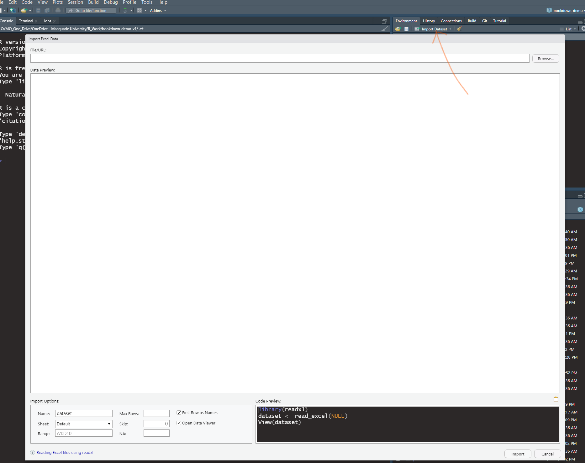
Figure 2.2: Import Dataset wizard in RStudio
Function \(\mathtt{dim}\) can also be used to define an array by assigning dimensions to a vector.↩︎