Topic 10 Technical Analysis using R

10.1 Technical Analysis (TA) using R
Introduction to TA
- A good resource https://bookdown.org/kochiuyu/Technical-Analysis-with-R/
“Technical Analysis is the science of recording, usually in graphic form, the actual history of trading (price changes, volume of transactions, etc.) in a certain stock or in the averages and then deducing from that pictured history the probable future trend”(Edwards & Magee (1966))
TA is considered as one of the first Data Science techniques in Finance
10.2 Technical Charts
Here we will use the quantmod and TTR package to generate some Technical Charts. The data will be downloaded from Yahoo Finance.
10.2.1 Candlesticks and OHLC chart
As demonstrated in the previous chapter, R package quantmod can be used to download daily OHLC data (Open, High, Low and Close) with volume.
quantmod (https://www.quantmod.com/) also allows to import data from csv files.
# Run the following to download and save the data, same as the
# regression chapter. Only run if data requires update of different
# assets are used
library(quantmod)
library(pander)
# download stock
BHP = getSymbols("BHP.AX", from = "2019-01-01", to = "2021-07-31", auto.assign = FALSE)
# download index
ASX = getSymbols("^AXJO", from = "2019-01-01", to = "2021-07-31", auto.assign = FALSE)
# save both in rds (to be used in the TA chapter)
saveRDS(BHP, file = "data/bhp_prices.rds")
saveRDS(ASX, file = "data/asx200.rds")library(quantmod)
library(pander)
BHP = readRDS("data/bhp_prices.rds")
ASX = readRDS("data/asx200.rds")
pander(head(BHP), caption = "OHLC Data", split.table = Inf)| Period | BHP.AX.Open | BHP.AX.High | BHP.AX.Low | BHP.AX.Close | BHP.AX.Volume | BHP.AX.Adjusted |
|---|---|---|---|---|---|---|
| 2019/01/02 12:00:00 AM | 34.28 | 34.55 | 33.65 | 33.68 | 7290354 | 26.68 |
| 2019/01/03 12:00:00 AM | 33.88 | 34.13 | 33.56 | 33.68 | 8473568 | 26.68 |
| 2019/01/04 12:00:00 AM | 33.1 | 33.39 | 32.96 | 33.38 | 9314513 | 26.44 |
| 2019/01/07 12:00:00 AM | 34.5 | 34.55 | 34.28 | 34.39 | 8553510 | 27.24 |
| 2019/01/08 12:00:00 AM | 34.6 | 34.68 | 34.43 | 34.43 | 8685056 | 27.28 |
| 2019/01/09 12:00:00 AM | 34.5 | 34.59 | 34.19 | 34.3 | 9459525 | 27.17 |
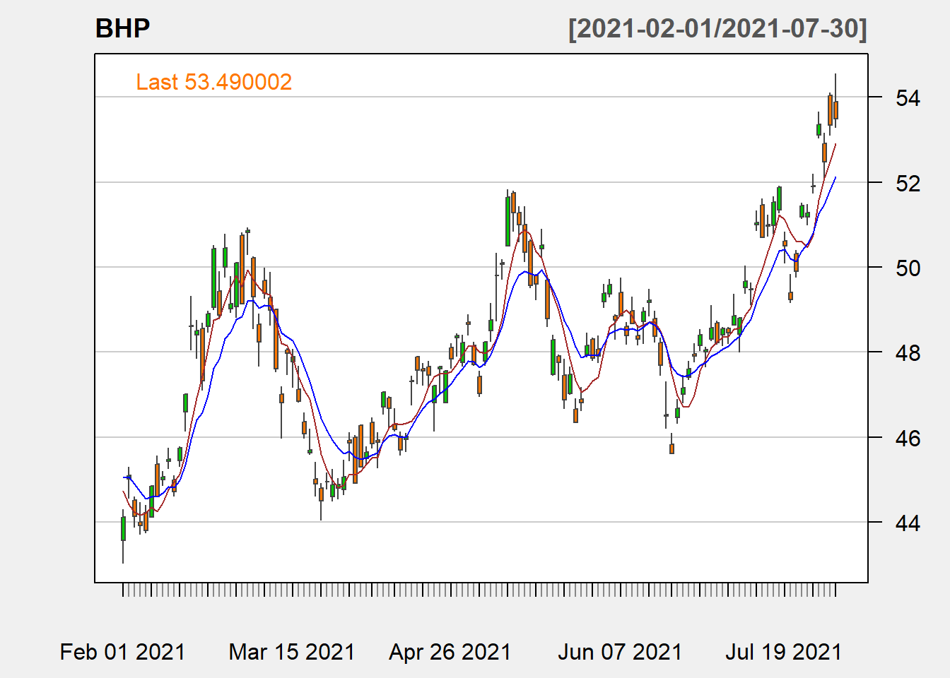
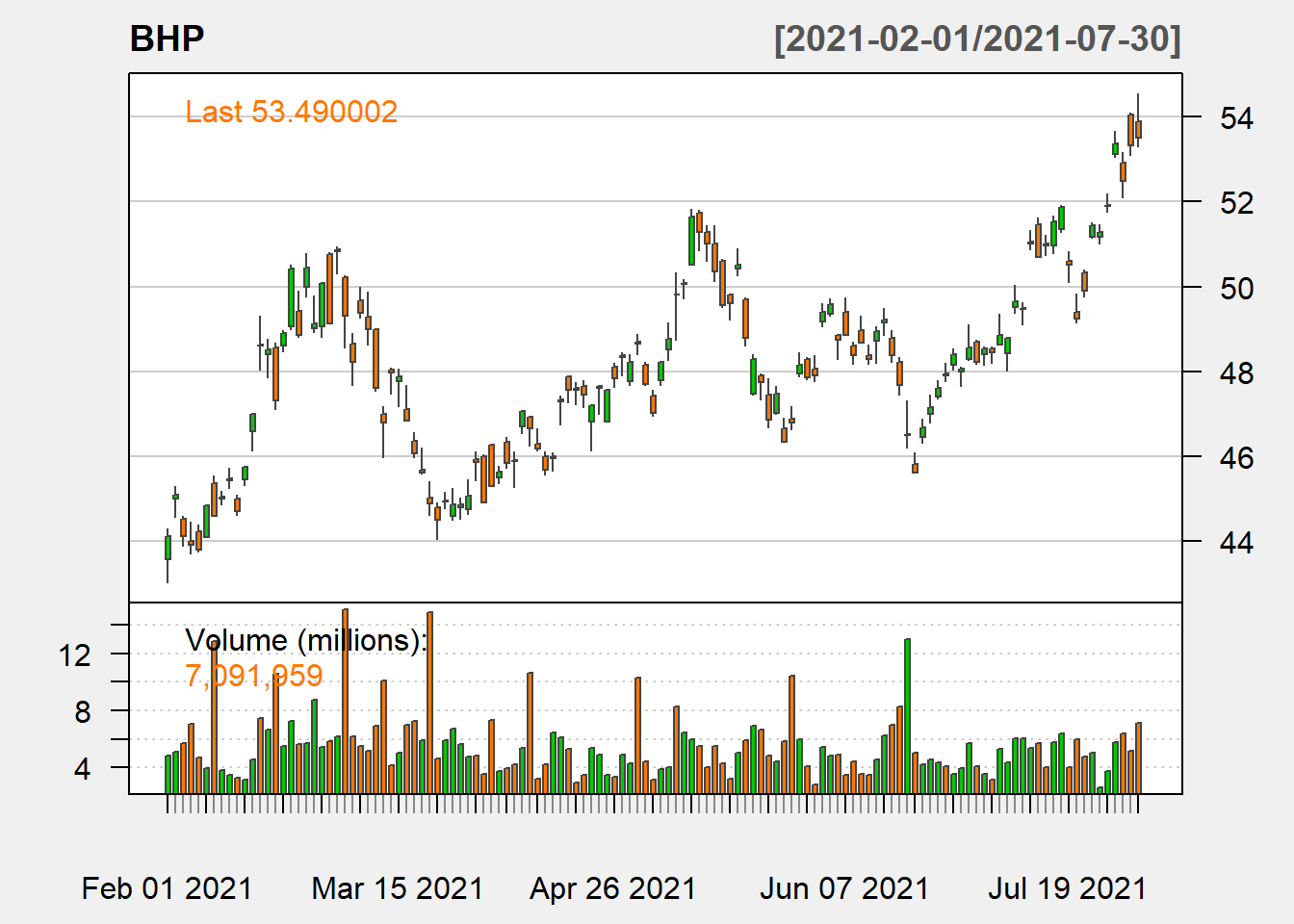
chartSeries(BHP, theme = "white")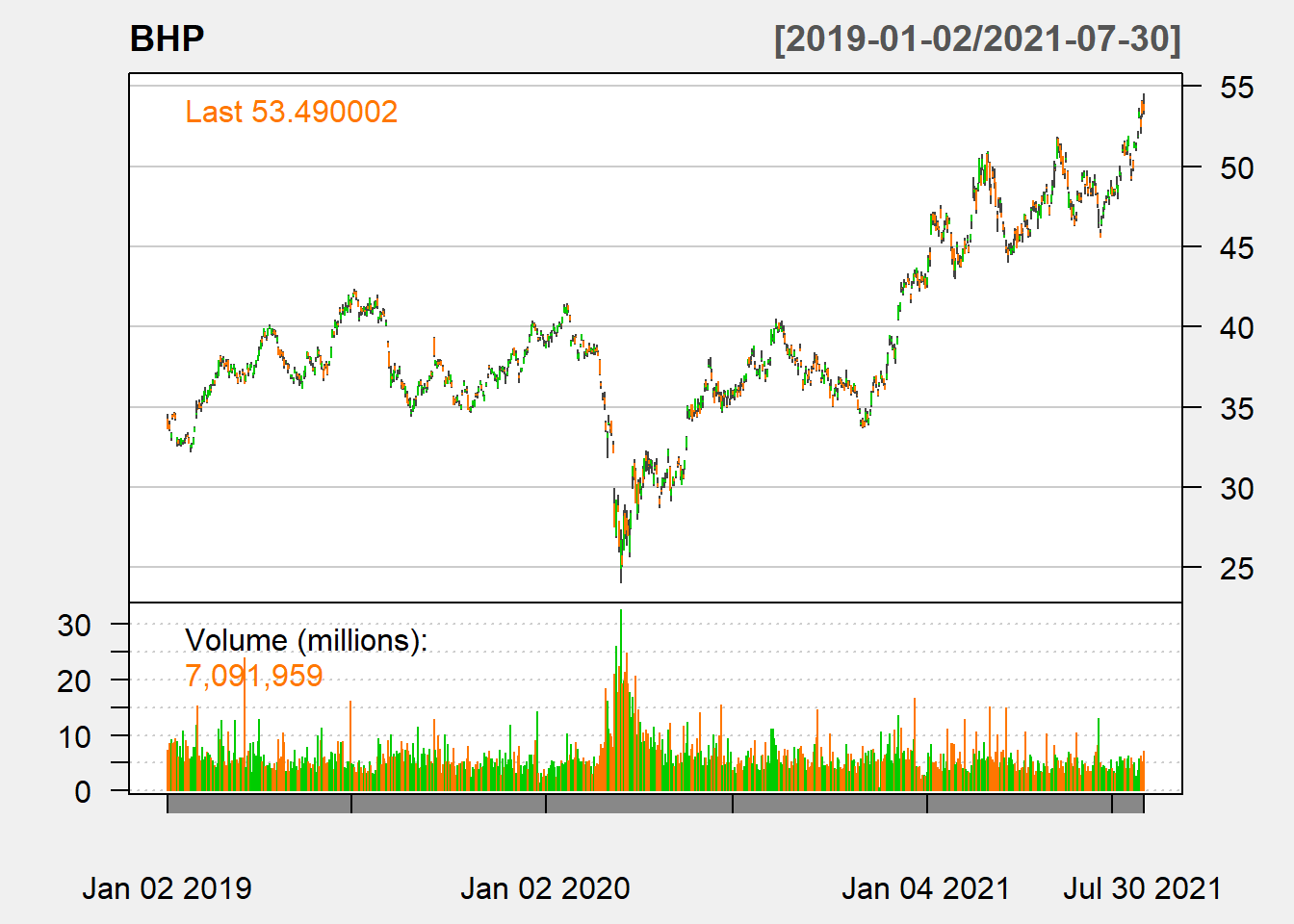
Figure 10.1: BHP Line Chart with Volume
addTA(ASX$AXJO.Close, col = "darkblue")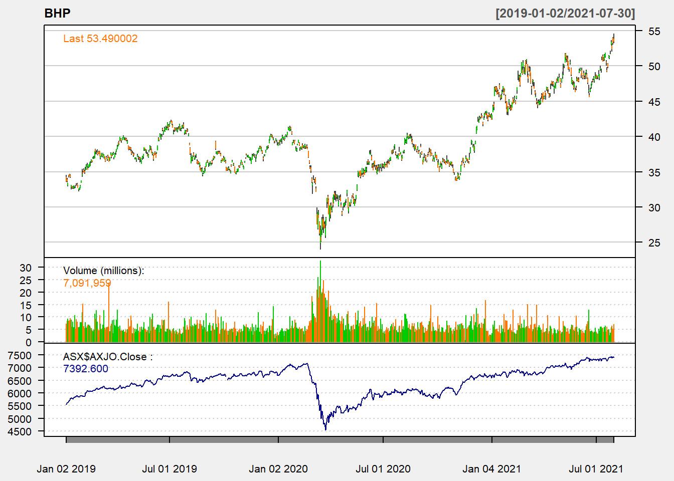
Figure 10.2: BHP and ASX
10.2.2 Line chart
chartSeries(BHP, type = "line", subset = "2020", theme = "white")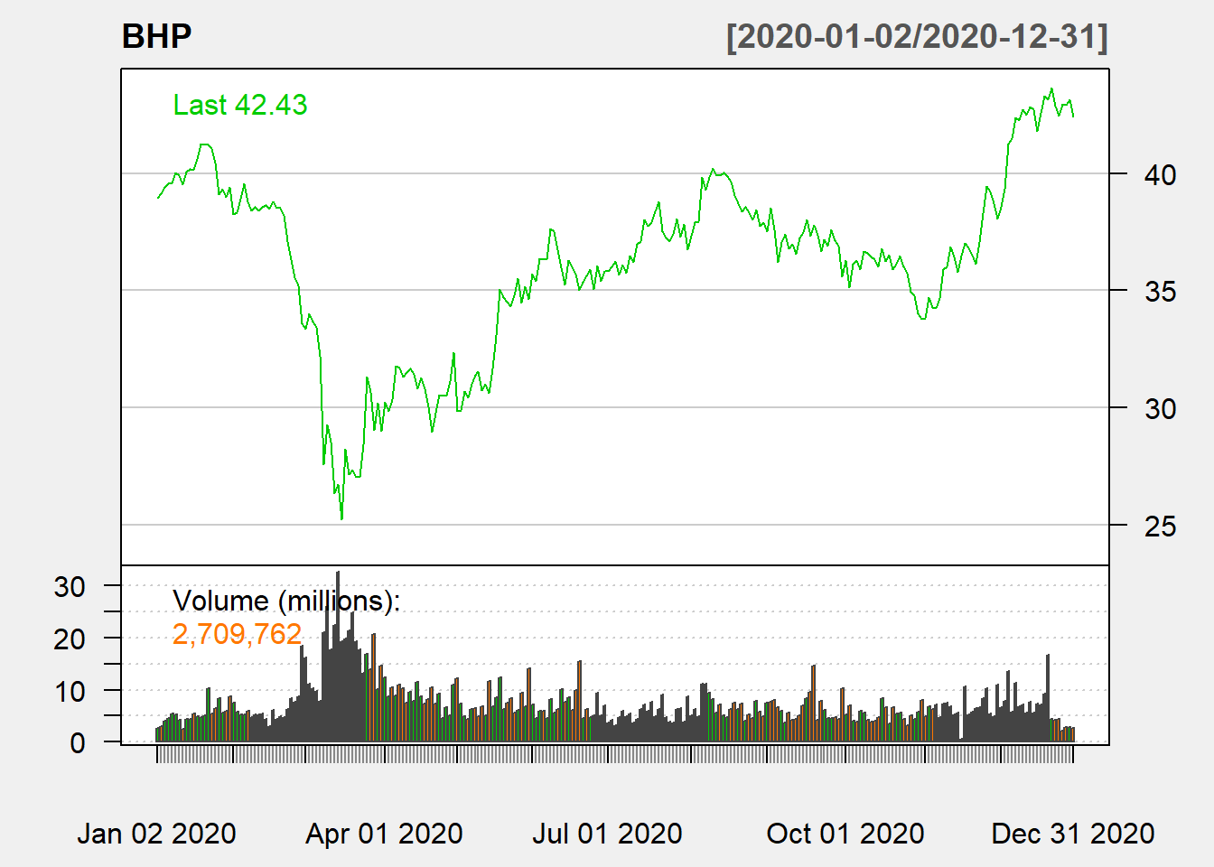
Figure 5.2: Line Chart
10.2.3 Candlestick chart
chartSeries(BHP, type = "candle", subset = "last 1 month", theme = "white")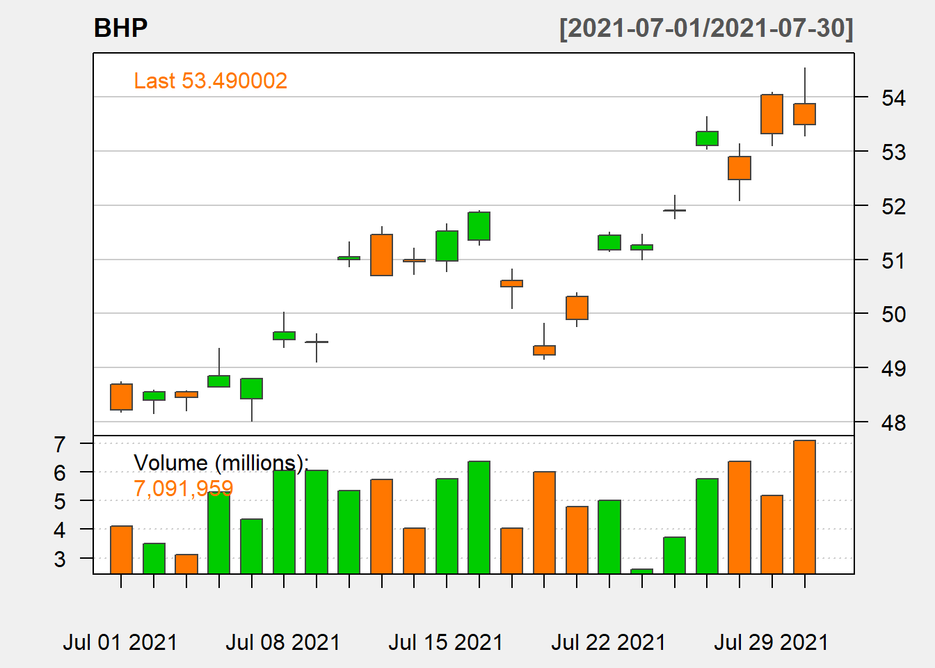
Figure 5.3: Candle Stick chart
Topic 11 Forecasting VaR using GARCH Models
11.1 Value at Risk
- Value at Risk (VaR) is the most widely used market risk measure in financial risk management and it is also used by practitioners such as portfolio managers to account for future market risk. VaR can be defined as loss in market value of an asset over a given time period that is exceeded with a probability \(\theta\). For a time series of returns \(r_{t}\) , \(VaR_{t}\) would be such that
\[\begin{equation} P[r_{t}<-VaR_{t}[I_{t-1}]=\theta \tag{11.1} \end{equation}\]
where \(I_{t-1}\) represents the information set at time t-1.
- Despite the appealing simplicity of VaR in its offering of a simple summary of the downside risk of an asset portfolio, there is no single way to calculate it (see Manganelli & Engle (2001) ) for an overview on VaR methods in finance).
1% VaR
- Convert the prices to returns
library(ggplot2)
# calculate normal density for the returns

# prices to returns

bhp2 = BHP$BHP.AX.Close
# covert to returns

bhp_ret = dailyReturn(bhp2, type = "log")
den1_r = coredata(bhp_ret)
den1_bhp = dnorm(x = den1_r, mean = mean(den1_r), sd = sd(den1_r))
data_rd = data.frame(den1_r, den1_bhp)
# change column names
colnames(data_rd) = c("x", "y")
# normal quantile
var1 = quantile(den1_r, 0.01)
p3 = ggplot(data_rd, aes(x = x, y = y)) + geom_line(size = 2) + geom_vline(xintercept = var1,
    lty = 2, col = "red", size = 2) + theme_bw() + labs(title = "Normal Distribution and 1% (Empirical) VaR")
p3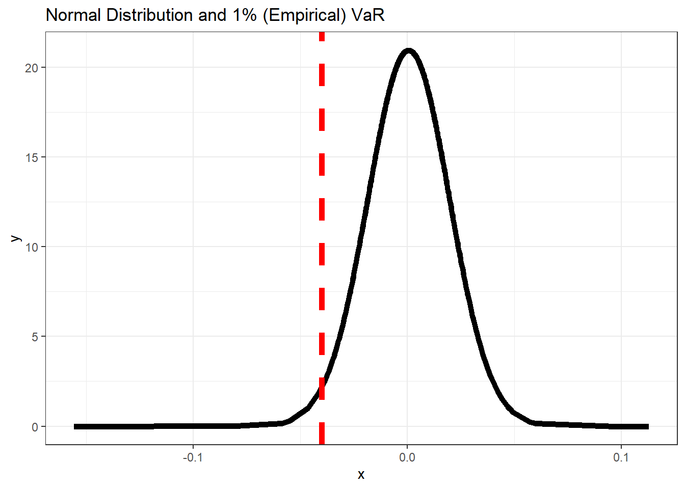
Figure 11.1: 1% VaR
- In distribution terms, for a distribution F, VaR can be defined as its p-th quantile given by
\[\begin{equation} VaR_{p}(V_{p})=F^{-1}(1-p) \tag{11.2} \end{equation}\]
where \(F^{-1}\) is the inverse of the distribution function also called as the quantile function. Hence VaR is easy to calculate once a distribution for the return series can be defined.
- VaR is the q-th quantile of the distribution of over a time horizon t, which is a well accepted measure of risk in financial management.
11.2 Volatility Modelling & Forecasting using GARCH
The Generalised Autoregressive Conditional Heteroskedasticity (GARCH) models (Bollerslev (1986), R. F. Engle (1982); R. Engle (2001)), most popular time series models used for forecasting conditional volatiltiy.
These models are conditional heteroskedastic as they take into account the conditional variance in a time series. GARCH models are one of the most widely used models for forecasting financial risk measures like VaR and Conditional VaR in financial risk modelling and management.
The GARCH models are a generalised version of ARCH models. A standard ARCH(p) process with p lag terms designed to capture volatility clustering can be written as follows
\[\begin{equation} \sigma_{t}^{2}=\omega+\sum_{i=1}^{p}\alpha_{i}Y_{t-i}^{2} \tag{11.3} \end{equation}\]
where the return on day t, is \(Y_{t}=\sigma_{t}Z_{t}\) and \(Z_{t}\sim i.i.d(0,1)\), i.e., the innovation in returns are driven by random shocks
- The GARCH(p,q) model include lagged volatility in an ARCH(p) model to incorporate the impact of historical returns which can be written as follows
\[\begin{equation} \sigma_{t}^{2}=\omega+\sum_{i=1}^{p}\alpha_{i}Y_{t-i}^{2}+\sum_{j=1}^{q}\beta_{j}\sigma_{t-j}^{2} \tag{11.4} \end{equation}\]
- GARCH(1,1) which employs only one lag per order, is the most common version used in empirical research and analysis.
11.3 GARCH(1,1) to forecast VaR
One of the most versatile and capable of them is the rugarch package. Here we use previously introduced asx_ret.RData dataset to demonstrate modelling GARCH using the functions and methods av ailable in the rugarch package.
Fitting a GARCH model using the rugarch package requires setting the model specification using the
ugarchspecfunction.A GARCH(1,1) model with a contant mean equation
mean.model=list(armaOrder=c(0,0)can be specified as follows:
library(rugarch)
garch_spec = ugarchspec(variance.model = list(model = "sGARCH", garchOrder = c(1,
1)), mean.model = list(armaOrder = c(0, 0)))- The above specification stored in
garch_speccan now be used to fit the GARCH(1,1) model to our data. The following code fits the GARCH(1,1) model to BHP log returns using the function and shows the results.
fit_garch = ugarchfit(spec = garch_spec, data = bhp_ret)
# show the estimates and other diagnostic tests
fit_garch
*---------------------------------*
*          GARCH Model Fit        *
*---------------------------------*

Conditional Variance Dynamics
-----------------------------------
GARCH Model : sGARCH(1,1)
Mean Model  : ARFIMA(0,0,0)
Distribution    : norm

Optimal Parameters
------------------------------------
        Estimate  Std. Error  t value Pr(>|t|)
mu      0.000929    0.000590   1.5733 0.115648
omega   0.000022    0.000011   1.9495 0.051231
alpha1  0.190305    0.061330   3.1029 0.001916
beta1   0.754359    0.082123   9.1857 0.000000

Robust Standard Errors:
        Estimate  Std. Error  t value Pr(>|t|)
mu      0.000929    0.000606   1.5338 0.125072
omega   0.000022    0.000018   1.2469 0.212446
alpha1  0.190305    0.142428   1.3361 0.181501
beta1   0.754359    0.157071   4.8027 0.000002

LogLikelihood : 1747.092

Information Criteria
------------------------------------

Akaike       -5.3306
Bayes        -5.3031
Shibata      -5.3306
Hannan-Quinn -5.3199

Weighted Ljung-Box Test on Standardized Residuals
------------------------------------
                        statistic p-value
Lag[1]                    0.03488  0.8518
Lag[2*(p+q)+(p+q)-1][2]   0.62736  0.6367
Lag[4*(p+q)+(p+q)-1][5]   1.62615  0.7089
d.o.f=0
H0 : No serial correlation

Weighted Ljung-Box Test on Standardized Squared Residuals
------------------------------------
                        statistic p-value
Lag[1]                     0.5304  0.4665
Lag[2*(p+q)+(p+q)-1][5]    2.1141  0.5917
Lag[4*(p+q)+(p+q)-1][9]    6.4221  0.2526
d.o.f=2

Weighted ARCH LM Tests
------------------------------------
            Statistic Shape Scale P-Value
ARCH Lag[3]    0.8395 0.500 2.000  0.3595
ARCH Lag[5]    1.3927 1.440 1.667  0.6210
ARCH Lag[7]    6.1375 2.315 1.543  0.1323

Nyblom stability test
------------------------------------
Joint Statistic:  0.5677
Individual Statistics:
mu     0.06882
omega  0.28626
alpha1 0.15743
beta1  0.19222

Asymptotic Critical Values (10% 5% 1%)
Joint Statistic:         1.07 1.24 1.6
Individual Statistic:    0.35 0.47 0.75

Sign Bias Test
------------------------------------
                   t-value   prob sig
Sign Bias           0.2418 0.8090
Negative Sign Bias  1.3289 0.1844
Positive Sign Bias  0.1904 0.8491
Joint Effect        2.9075 0.4061


Adjusted Pearson Goodness-of-Fit Test:
------------------------------------
  group statistic p-value(g-1)
1    20     22.45       0.2623
2    30     31.69       0.3337
3    40     48.63       0.1388
4    50     54.41       0.2761


Elapsed time : 0.1552448 - Selected fitted statistics can be obtained using various methods available to the
ugarchfitobject class
par1 = par()  #save graphic parameters

par(mfrow = c(1, 2))
# generate plots using the which argument Figure-12 1. ACF of
# standardised residuals
plot(fit_garch, which = 10)
# 2. Conditional SD (vs |returns|)
plot(fit_garch, which = 3)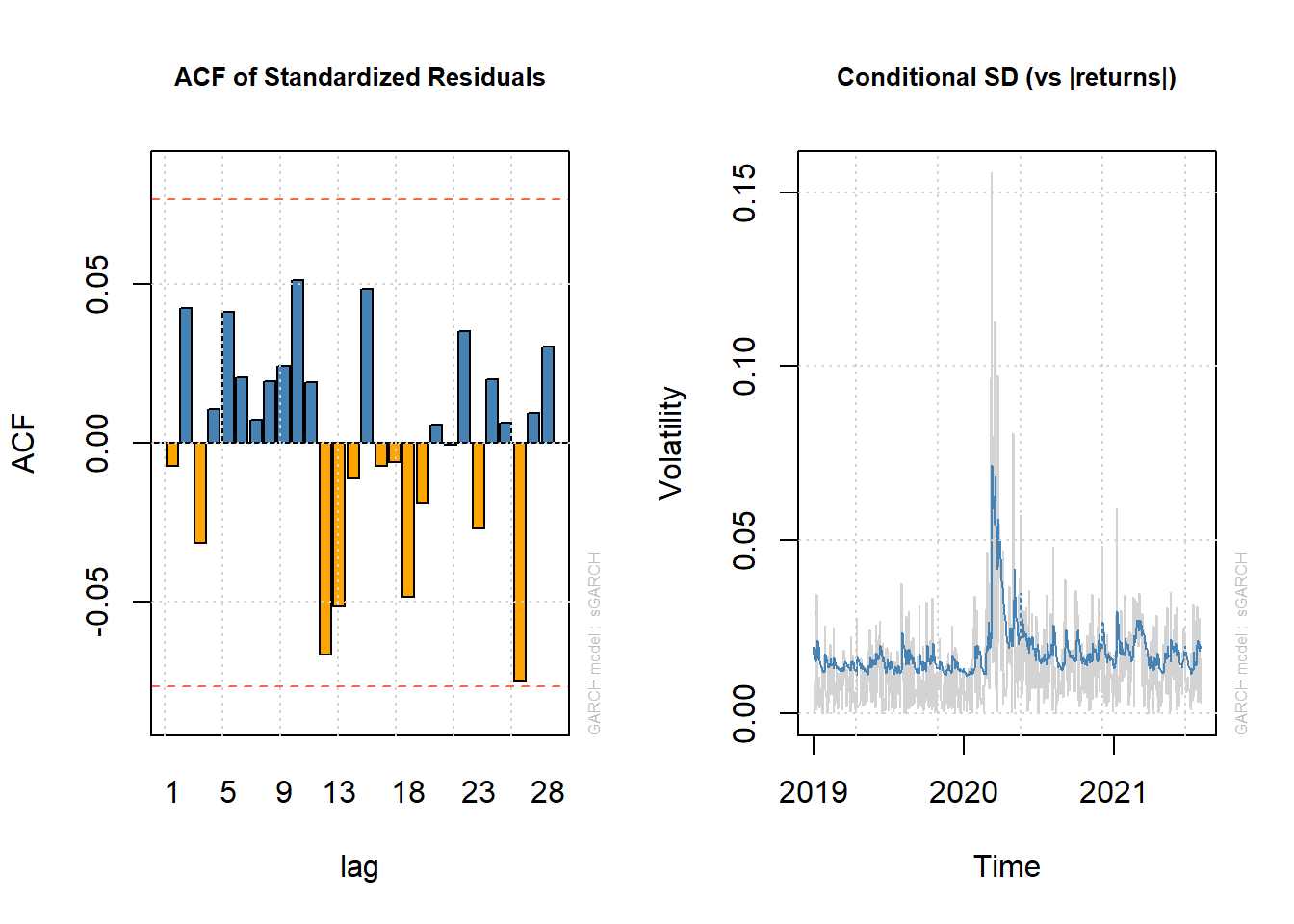
Figure 11.2: Two Informative Plots for GARCH(1,1)
11.4 VaR forecasts using out of sample
- Let’s use Student-t distribution as Financial Returns don’t always follow normal distribution
# spec2 with student-t distribution
spec2 = ugarchspec(variance.model = list(model = "sGARCH", garchOrder = c(1,
1)), mean.model = list(armaOrder = c(0, 0)), distribution.model = "std")- The rugarch package has a very useful function for estimating moving window models and forecasting VaR. The function provides method for creating rolling forecasts from GARCH models and has various arguments to specify the forecast length (), window size (), model refitting frequency (), a rolling or recursive estimation window () etc.
var.t = ugarchroll(spec2, data = bhp_ret, n.ahead = 1, forecast.length = ndays(bhp_ret) -
    500, refit.every = 5, window.size = 500, refit.window = "rolling",
calculate.VaR = TRUE, VaR.alpha = c(0.01, 0.05))- We can plot the 1% and 5% VaR forecasts against the actual returns using the following routine.
# note the plot method provides four plots with option-4 for the VaR
# forecasts 1% Student-t GARCH VaR
par(mfrow = c(1, 2))
plot(var.t, which = 4, VaR.alpha = 0.01)
# 5% Student-t GARCH VaR
plot(var.t, which = 4, VaR.alpha = 0.05)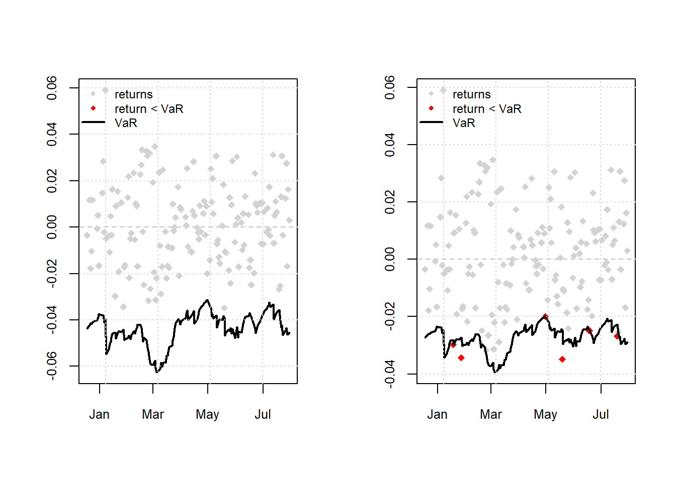
Figure 11.3: Actual Return Vs 1% VaR forecasts
- Finally backtesting can be obtained using the
reportmethod
# backtest for VaR forecasts

report(var.t, VaR.alpha = 0.05)  #default value of alpha is 0.01
VaR Backtest Report
===========================================
Model: sGARCH-std
Backtest Length: 154
Data:
==========================================
alpha: 5%
Expected Exceed: 7.7
Actual VaR Exceed: 6
Actual %: 3.9%
Unconditional Coverage (Kupiec)
Null-Hypothesis: Correct Exceedances
LR.uc Statistic: 0.426
LR.uc Critical: 3.841
LR.uc p-value: 0.514
Reject Null: NO
Conditional Coverage (Christoffersen)
Null-Hypothesis: Correct Exceedances and
Independence of Failures
LR.cc Statistic: 0.916
LR.cc Critical: 5.991
LR.cc p-value: 0.633
Reject Null: NO